Getting Started with the HHS Medicaid Provider Spending Dataset

How to setup your own local database

In February 2026, the US Department of Health & Human Services (HHS) released a data file containing Medicaid monthly spending for outpatient and professional claims by provider and HCPCS code from 2018-2024 across the entire United States. It’s a pretty massive dataset (~238M rows), so being able to set it up to efficiently explore it on your own machine takes a little bit of care. This article is meant to show you how to set up a basic data model from a few different important sources to be able to conduct useful analysis using some cool frameworks I was first exposed to along the way. Specifically, this guide is more so scoped around the assumption that you want to conduct analysis for a specific state (in my case, Wisconsin) as to reduce the data size you have to work with. But you could apply this to any state of your choosing, or try to build the data model for the entire country.

Note that all code will be written in the R environment.

First, an app

To start things off, I’ll showcase what I’ve been building with this dataset:

It is an R Shiny application exploring Medicaid spending for the state of Wisconsin that is hosted on Posit Connect Cloud. You can access the live app here and the source code here.

I won’t go into a ton of detail about the specifics of everything in there, but feel free to go and try it out. It’s certainly very fun and interesting data to explore. There are filters to search by individual providers and codes, conduct provider-level or code-level analysis, and download your selected dataset. My suggestion would be to first read through the About tab so you can understand more context about what is (and isn’t included) and how to use it.

Now to the data model 👇

Accessing the dataset

The first step is to of course go and download the Medcaid spending data file from the HHS Open Data Platform. When you go to the webpage, click the drop-down arrow in the upper-right to see the download options:

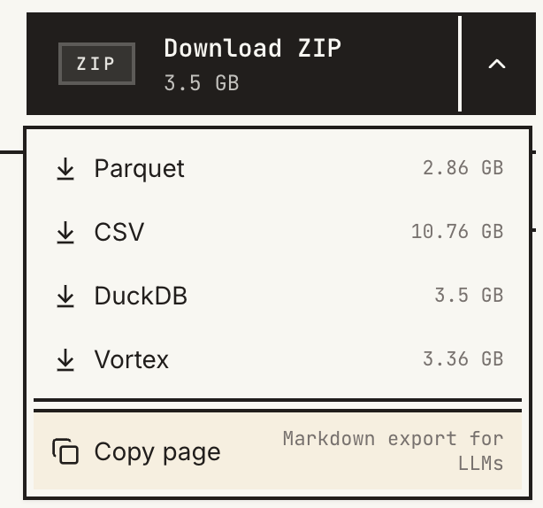
As I learned along the way, I would not advise using the .csv file (just look at those size differences!). Instead, I opted to use the .duckdb file as my primary source, though I’ve never used DuckDB before. I also downloaded the .parquet file for comparison, but never used those file types either. Turns out these are both extremely useful frameworks to learn to process and work with (particularly large) data. In fact, they go really well together as well.

Setup your environment

Before we go any further, make sure you have the required packages installed to begin working with this data in R:

# Install the packages
install.packages("DBI")
install.packages("duckdb")

Now let’s take your downloaded .duckdb file and put it in an assumed directory structure, like:

- data/
  + medicaid-provider-spending.duckdb

We’ll assume that data is some folder on your machine that contains the dataset (which we’ll add more stuff to later). I’m also assuming this is the name of the downloaded file, but rename it if necessary. Now let’s just create an R variable that points to this directory. For example,

root <- "/path/to/my/data"

Now if you run list.files() you should see your file within root (note that I used stringr::str_subset() here because I already have other files in my directory, but you don’t need that part):

list.files(root) |> 

  # Filtering to ignore other files
  stringr::str_subset("medicaid-provider-spending[.]duckdb")

[1] "medicaid-provider-spending.duckdb"

A first glance

Now let’s just take a peek under the hood and get the mechanics working with the duckdb package. In short, DuckDB is a SQL database that runs very efficiently wherever you are executing your code (e.g., so instead of needing a full database setup, you can literally just have a database sitting in a file and write queries against it, among many other possibilities). We’ll start by just loading the packages and looking at what’s inside our .duckdb file.

# Load packages
library(DBI)
library(duckdb)
library(tidyverse)

# Connect to the database
con <- dbConnect(duckdb::duckdb(), paste0(root, "/medicaid-provider-spending.duckdb"))

# List tables
dbListTables(con)

[1] "dataset"

The dbListTables() function list the tables in our database. There’s only one (1) and it’s called dataset. Now we can assess the columns in the table:

# Get schema info
dbGetQuery(con, "DESCRIBE dataset")

                 column_name column_type null  key default extra
1   BILLING_PROVIDER_NPI_NUM     VARCHAR  YES <NA>    <NA>  <NA>
2 SERVICING_PROVIDER_NPI_NUM     VARCHAR  YES <NA>    <NA>  <NA>
3                 HCPCS_CODE     VARCHAR  YES <NA>    <NA>  <NA>
4           CLAIM_FROM_MONTH     VARCHAR  YES <NA>    <NA>  <NA>
5             TOTAL_PATIENTS      BIGINT  YES <NA>    <NA>  <NA>
6          TOTAL_CLAIM_LINES      BIGINT  YES <NA>    <NA>  <NA>
7                 TOTAL_PAID      DOUBLE  YES <NA>    <NA>  <NA>

Just as the website describes, we have rows that show numeric summaries such as monthly total paid amount, claims lines, and unique patients by HCPCS code for combinations of who the billing and servicing providers were. Let’s look at some of the actual data:

# Select 10 rows of data to view
dbGetQuery(con, "SELECT * FROM dataset LIMIT 10") |> as_tibble()

# A tibble: 10 × 7
   BILLING_PROVIDER_NPI_NUM SERVICING_PROVIDER_NPI…¹ HCPCS_CODE CLAIM_FROM_MONTH
   <chr>                    <chr>                    <chr>      <chr>           
 1 <NA>                     5200000300               20         2018-06         
 2 <NA>                     5200000300               20         2018-01         
 3 <NA>                     5200000300               20         2018-02         
 4 <NA>                     5200000300               20         2019-10         
 5 <NA>                     5200000300               20         2018-08         
 6 <NA>                     5200000300               20         2019-11         
 7 <NA>                     5200000300               20         2019-12         
 8 <NA>                     5200000300               20         2019-06         
 9 <NA>                     5200000300               20         2018-09         
10 <NA>                     5200000300               20         2019-04         
# ℹ abbreviated name: ¹​SERVICING_PROVIDER_NPI_NUM
# ℹ 3 more variables: TOTAL_PATIENTS <dbl>, TOTAL_CLAIM_LINES <dbl>,
#   TOTAL_PAID <dbl>

Finally, let’s take a look some overall dataset summaries such as the number of records and the total dollar amount represented in the dataset:

# Row count + paid amount total
dbGetQuery(
  con,
  "SELECT COUNT(1) AS RowCount, SUM(TOTAL_PAID) AS TotalPaid FROM dataset"
) |>

  # Format the result
  mutate(
    RowCount = scales::comma(RowCount),
    TotalPaid = scales::dollar(TotalPaid)
  ) |>

  # Make a clean table
  knitr::kable(format = "html") |>
  kableExtra::kable_styling()

RowCount	TotalPaid
238,015,729	$21,799,399,688,550

An initial filter

One thing you’ll notice is that the dollar amount totals are enormous (~$21T). Upon further research, this total is way more than would be expected over this time period for outpatient and professional claims. And indeed in the Examples tab of the source website, their analysis only pertains to rows where the billing and provider NPI number are present. This gives us a hunch that we probably need to filter some stuff out.

Deeper evaluation

Let’s explore these counts/totals by whether or not both providers are listed or not.

dbGetQuery(
  con,
  "SELECT 
      CASE WHEN 
        BILLING_PROVIDER_NPI_NUM IS NULL OR SERVICING_PROVIDER_NPI_NUM IS NULL THEN 'One missing'
        ELSE 'Both Present'
      END AS RowStatus,
      COUNT(1) AS RowCount, 
      SUM(TOTAL_PAID) AS TotalPaid 
    FROM dataset
    GROUP BY 
    CASE WHEN 
        BILLING_PROVIDER_NPI_NUM IS NULL OR SERVICING_PROVIDER_NPI_NUM IS NULL THEN 'One missing'
        ELSE 'Both Present'
      END"
) |>

  # Format the result
  mutate(
    RowCount = scales::comma(RowCount),
    TotalPaid = scales::dollar(TotalPaid)
  ) |>

  # Make a clean table
  knitr::kable(format = "html") |>
  kableExtra::kable_styling()

RowStatus	RowCount	TotalPaid
Both Present	221,375,333	$1,003,056,531,504
One missing	16,640,396	$20,796,343,157,071

We can see that virtually all (~95%) of the total dollar amount is captured by rows where at least one (1) provider is missing, yet these rows account for a small subset of the total number of rows. So there must be other things, like capitation costs, included in these rows that are not of interest, and causes dollar amounts for distinct events we’re interested in to be inflated.

On the contrary, the rows where both providers are present (which is most rows) have a total of ~$1T in spending, which is a more reasonable estimate for claims paid to providers over this time period given the context.

Given this discovery, and the fact that the examples also only use these rows, we are only going to work with a filtered subset of this data.

dbGetQuery(
  con,
  "SELECT 
    COUNT(1) AS RowCount, 
    SUM(TOTAL_PAID) AS TotalPaid 
    FROM dataset 
    WHERE 
      BILLING_PROVIDER_NPI_NUM IS NOT NULL AND 
      SERVICING_PROVIDER_NPI_NUM IS NOT NULL"
) 

   RowCount    TotalPaid
1 221375333 1.003057e+12

This row subset will be our claims basis for the data model setup.

Let’s go ahead and close our current connection to the database (for now), and we’ll come back to it later.

# Close the connection
dbDisconnect(con, shutdown = TRUE)

Building the local database

Given our exploratory work up to this point, we have somewhat of a strategy to make our own local database. However, as we’ll see, to make it state-specific (e.g., Wisconsin only) there will be other data sources we’ll need to bring in along the way to make it happen.

Initializing the database

We are going to start off by simply initializing a new DuckDB database in our data directory. This will be an empty database but makes it available for us to write to.

# Initialize a new database (creates it if it doesn't exist)
my_db <- dbConnect(duckdb::duckdb(), paste0(root, "/wisconsin_medicaid_database.duckdb"))

# Check for tables
dbListTables(my_db)

[1] "claims" "codes"  "npi_wi"

Defining the geography through providers

The first thing we’re going to add to our database is not the claims data, because that doesn’t have geographic indicators associated with it. What we need to do is find a lookup table for the NPI numbers so that we can define our tables for providers from the state of Wisconsin only.

Goal: Build a lookup table containing providers who primarily practice in the state of Wisconsin.

Identifying the providers data

We can use the NPPES NPI Files that are made available by CMS. Once you go to that page, look for the Monthly NPPES Downloadable File Version 2 (V.2) and download the .zip file. Once that is downloaded, there are numerous files in there such as .pdf (giving file/field descriptions), and _fileheader.csv files that provide you with what the top row of column names look like (so you can open it without trying to open the full dataset). The file we are interested in is npidata_pfile_20050523-20260412.csv. Note: Your file name may be different depending on the date you downloaded it.

Warning

This dataset is massive (~11.3GB). I would recommend not trying to open it directly on your computer.

Place the file in your data directory. Your folder should look something like this now:

- data/
  + medicaid-provider-spending.duckdb
  + wisconsin_medicaid_database.duckdb
  + npidata_pfile_20050523-20260412.csv

Developing a clean table

This is very wide data (check the companion _fileheader.csv file to see all the columns). Now we need figure out which ones we should select to make a smaller, more manageable table for our use. But first, how are we actually going to access this dataset?

DuckDB magic

Instead of importing the entire 11GB file into memory (e.g., through readr::read_csv()), we can use duckdb to access the .csv file via SQL. For example, let’s look at the first 10 rows of the data:

dbGetQuery(
  my_db,
  paste0('
    SELECT *
    FROM read_csv_auto("', root, '/npidata_pfile_20050523-20260412.csv")
    LIMIT 10'
  )
) |> as_tibble()

# A tibble: 10 × 330
          NPI `Entity Type Code` `Replacement NPI` Employer Identification Num…¹
        <dbl>              <dbl>             <dbl> <chr>                        
 1 1679576722                  1                NA <NA>                         
 2 1588667638                  1                NA <NA>                         
 3 1497758544                  2                NA <UNAVAIL>                    
 4 1306849450                 NA                NA <NA>                         
 5 1215930367                  1                NA <NA>                         
 6 1023011178                  2                NA <UNAVAIL>                    
 7 1932102084                  1                NA <NA>                         
 8 1841293990                  1                NA <NA>                         
 9 1750384806                  1                NA <NA>                         
10 1669475711                  1                NA <NA>                         
# ℹ abbreviated name: ¹​`Employer Identification Number (EIN)`
# ℹ 326 more variables:
#   `Provider Organization Name (Legal Business Name)` <chr>,
#   `Provider Last Name (Legal Name)` <chr>, `Provider First Name` <chr>,
#   `Provider Middle Name` <chr>, `Provider Name Prefix Text` <chr>,
#   `Provider Name Suffix Text` <chr>, `Provider Credential Text` <chr>,
#   `Provider Other Organization Name` <chr>, …

We use the read_csv_auto function native to DuckDB to run queries on our data file directly (without pulling the whole thing into memory). We can see there are 330 columns, but we only want a small subset of those for our purposes.

Selecting relevant columns

After researching and reviewing the documentation, I found that the following columns capture enough relevant information.

dbGetQuery(
  my_db,
  paste0('
    SELECT
      CAST("NPI" AS VARCHAR) AS NPI,
      "Entity Type Code" AS EntityType,
      "Provider Organization Name (Legal Business Name)" AS Organization,
      "Provider Last Name (Legal Name)" AS LastName,
      "Provider First Name" AS FirstName,
      "Provider Sex Code" AS Sex,
      "Provider Credential Text" AS Credentials,
      "Provider First Line Business Practice Location Address" AS Address,
      "Provider Business Practice Location Address City Name" AS City,
      "Provider Business Practice Location Address State Name" AS State,
      "Provider Business Practice Location Address Postal Code" AS Zip,
      "Healthcare Provider Taxonomy Code_1" AS TaxonomyCode,
      "Is Organization Subpart" AS OrganizationSubpart,
      "Last Update Date" AS LastUpdateDate,
      "NPI Deactivation Date" AS DeactivationDate,
      "NPI Reactivation Date" AS ReactivationDate
    FROM read_csv_auto("', root, '/npidata_pfile_20050523-20260412.csv")
    LIMIT 10'
  )
) |> as_tibble()

# A tibble: 10 × 16
   NPI      EntityType Organization LastName FirstName Sex   Credentials Address
   <chr>         <dbl> <chr>        <chr>    <chr>     <chr> <chr>       <chr>  
 1 1679576…          1 <NA>         WIEBE    DAVID     M     M.D.        3500 C…
 2 1588667…          1 <NA>         PILCHER  WILLIAM   M     MD          1824 K…
 3 1497758…          2 CUMBERLAND … <NA>     <NA>      <NA>  <NA>        3418 V…
 4 1306849…         NA <NA>         <NA>     <NA>      <NA>  <NA>        <NA>   
 5 1215930…          1 <NA>         GRESSOT  LAURENT   M     M.D.        17323 …
 6 1023011…          2 COLLABRIA C… <NA>     <NA>      <NA>  <NA>        414 S …
 7 1932102…          1 <NA>         ADUSUMI… RAVI      M     MD          2940 N…
 8 1841293…          1 <NA>         WORTSMAN SUSAN     F     MA-CCC      425 E …
 9 1750384…          1 <NA>         BISBEE   ROBERT    M     MD          808 JO…
10 1669475…          1 <NA>         SUNG     BIN       F     M. D.       7629 T…
# ℹ 8 more variables: City <chr>, State <chr>, Zip <chr>, TaxonomyCode <chr>,
#   OrganizationSubpart <chr>, LastUpdateDate <date>, DeactivationDate <date>,
#   ReactivationDate <date>

Notice that I also renamed the columns to make them easier to work with (e.g., by removing whitespace).

Applying the state filter

The last, but most important, thing we need to do is to apply a relevant filter to only keep providers relevant to our scope (i.e., the state of Wisconsin). I determined that doing this based on the provider’s business practice location makes the most sense. So our final query looks like this:

dbGetQuery(
  my_db,
  paste0('
    SELECT
      CAST("NPI" AS VARCHAR) AS NPI,
      "Entity Type Code" AS EntityType,
      "Provider Organization Name (Legal Business Name)" AS Organization,
      "Provider Last Name (Legal Name)" AS LastName,
      "Provider First Name" AS FirstName,
      "Provider Sex Code" AS Sex,
      "Provider Credential Text" AS Credentials,
      "Provider First Line Business Practice Location Address" AS Address,
      "Provider Business Practice Location Address City Name" AS City,
      "Provider Business Practice Location Address State Name" AS State,
      "Provider Business Practice Location Address Postal Code" AS Zip,
      "Healthcare Provider Taxonomy Code_1" AS TaxonomyCode,
      "Is Organization Subpart" AS OrganizationSubpart,
      "Last Update Date" AS LastUpdateDate,
      "NPI Deactivation Date" AS DeactivationDate,
      "NPI Reactivation Date" AS ReactivationDate
    FROM read_csv_auto("', root, '/npidata_pfile_20050523-20260412.csv")
    WHERE "Provider Business Practice Location Address State Name" = \'WI\'
    LIMIT 10'
  )
) |> as_tibble()

# A tibble: 10 × 16
   NPI      EntityType Organization LastName FirstName Sex   Credentials Address
   <chr>         <dbl> <chr>        <chr>    <chr>     <chr> <chr>       <chr>  
 1 1871596…          1 <NA>         WOLTER   TIMOTHY   M     MD          716 W …
 2 1861495…          1 <NA>         LEA      ROBERT    M     MD          24509 …
 3 1881697…          2 FOX VALLEY … <NA>     <NA>      <NA>  <NA>        201 W …
 4 1053314…          1 <NA>         BOUSH    GEORGE    M     M.D.        123 HO…
 5 1508869…          1 <NA>         HAASCH   KATHLEEN  F     MS CCC-A F… 1442 N…
 6 1245233…          1 <NA>         GERING   KRISTIE   F     MD          2829 C…
 7 1699778…          2 CHIPPEWA VA… <NA>     <NA>      <NA>  <NA>        1200 O…
 8 1053314…          2 HOSPICE ALL… <NA>     <NA>      <NA>  <NA>        10220 …
 9 1922001…          1 <NA>         SCHOLL   PAUL      M     D.D.S       9211 W…
10 1255334…          1 <NA>         CONRADT  MARK      M     AU.D.       119 E …
# ℹ 8 more variables: City <chr>, State <chr>, Zip <chr>, TaxonomyCode <chr>,
#   OrganizationSubpart <chr>, LastUpdateDate <date>, DeactivationDate <date>,
#   ReactivationDate <date>

Note: Since we’re tying recent NPI files to historical claims, we may not get exact coverage as provider lists can change, but it gives us most of what we need for meaningful analysis.

Loading the providers to our database

Now we just need to slightly adjust our code to load the full result into the database instead of simply querying a result (i.e., use dbExecute(), add a CREATE TABLE statement, and remove the LIMIT 10):

if(!dbExistsTable(my_db, "npi_wi")) {
  dbExecute(
    my_db,
    paste0('
      CREATE TABLE npi_wi AS
      SELECT
        CAST("NPI" AS VARCHAR) AS NPI,
        "Entity Type Code" AS EntityType,
        "Provider Organization Name (Legal Business Name)" AS Organization,
        "Provider Last Name (Legal Name)" AS LastName,
        "Provider First Name" AS FirstName,
        "Provider Sex Code" AS Sex,
        "Provider Credential Text" AS Credentials,
        "Provider First Line Business Practice Location Address" AS Address,
        "Provider Business Practice Location Address City Name" AS City,
        "Provider Business Practice Location Address State Name" AS State,
        "Provider Business Practice Location Address Postal Code" AS Zip,
        "Healthcare Provider Taxonomy Code_1" AS TaxonomyCode,
        "Is Organization Subpart" AS OrganizationSubpart,
        "Last Update Date" AS LastUpdateDate,
        "NPI Deactivation Date" AS DeactivationDate,
        "NPI Reactivation Date" AS ReactivationDate
      FROM read_csv_auto("', root, '/npidata_pfile_20050523-20260412.csv")
      WHERE "Provider Business Practice Location Address State Name" = \'WI\'
      '
    )
  )
}

Note: We wrapped the table creation in dbExistsTable() so that it doesn’t have to re-write my table everytime my blog post is rendered.

Now if we look at the tables in our new database, we should see the providers table loaded.

dbListTables(my_db)

[1] "claims" "codes"  "npi_wi"

And we can start running queries against it:

# View the top 10 rows
dbGetQuery(
  my_db,
  "SELECT *
    FROM npi_wi 
    LIMIT 10"
) |> as_tibble()

# A tibble: 10 × 16
   NPI      EntityType Organization LastName FirstName Sex   Credentials Address
   <chr>         <dbl> <chr>        <chr>    <chr>     <chr> <chr>       <chr>  
 1 1871596…          1 <NA>         WOLTER   TIMOTHY   M     MD          716 W …
 2 1861495…          1 <NA>         LEA      ROBERT    M     MD          24509 …
 3 1881697…          2 FOX VALLEY … <NA>     <NA>      <NA>  <NA>        201 W …
 4 1053314…          1 <NA>         BOUSH    GEORGE    M     M.D.        123 HO…
 5 1508869…          1 <NA>         HAASCH   KATHLEEN  F     MS CCC-A F… 1442 N…
 6 1245233…          1 <NA>         GERING   KRISTIE   F     MD          2829 C…
 7 1699778…          2 CHIPPEWA VA… <NA>     <NA>      <NA>  <NA>        1200 O…
 8 1053314…          2 HOSPICE ALL… <NA>     <NA>      <NA>  <NA>        10220 …
 9 1922001…          1 <NA>         SCHOLL   PAUL      M     D.D.S       9211 W…
10 1255334…          1 <NA>         CONRADT  MARK      M     AU.D.       119 E …
# ℹ 8 more variables: City <chr>, State <chr>, Zip <chr>, TaxonomyCode <chr>,
#   OrganizationSubpart <chr>, LastUpdateDate <date>, DeactivationDate <date>,
#   ReactivationDate <date>

# Count the number of providers
dbGetQuery(
  my_db,
  "SELECT
      COUNT(1) AS RowCount,
      COUNT(DISTINCT NPI) AS UniqueProviders
    FROM npi_wi 
    LIMIT 10"
) |> as_tibble()

# A tibble: 1 × 2
  RowCount UniqueProviders
     <dbl>           <dbl>
1   139254          139254

Type 1 vs. Type 2 providers

You’ll notice in the npi_wi table that there is an EntityType column that takes on values 1 or 2. Additionally, for EntityType=1, the first/last name of an individual provider is populated. For EntityType=2, an organization name is populated. This field distinguishes between Type 1 and Type 2 providers (see details here). This is an important distinction to account for when analyzing this data. Often we’ll find that individuals (i.e., Type 1) will be listed as the servicing provider, and an organization (i.e., Type 2) will be listed as the billing provider, which generally means that the individual who provided the service works for a broader organization who actually did the billing (like a hospital).

Throughout the dataset you’ll find variations of claims where an individual or organization is listed as both the servicing and billing providers, or one of each. Keep this in mind when searching the database.

Loading the claims data

Now that we’ve restricted our provider list, we can now focus on loading the actual claims data into our database.

Goal: Create a claims database table filtered to only those in our derived Wisconsin NPI provider list

Cross-database attachment

One extremely cool feature of DuckDB is the native ability to easily allow different .duckdb databases to talk to one another within an exectured query. This is especially useful for us because our npi_wi table containing Wisconsin providers lives in our new database that we created, while the main Medicaid claims data lives in the .duckdb file we downloaded from HHS. Yet, we want to filter the latter to providers in the former. Luckiily, there’s an easy way to do this by just attaching an external table to our working database using ATTACH:

dbExecute(
  my_db, # <-- OUR database (not the one containing claims)
  paste0("ATTACH '", root, "/medicaid-provider-spending.duckdb' AS medicaid_src")
)

[1] 0

Now we can query this table from our database connection (my_db) by specifying the full database + schema name:

dbGetQuery(
  my_db,
  "
    SELECT *
    FROM medicaid_src.main.dataset
    LIMIT 10
  "
) |> as_tibble()

# A tibble: 10 × 7
   BILLING_PROVIDER_NPI_NUM SERVICING_PROVIDER_NPI…¹ HCPCS_CODE CLAIM_FROM_MONTH
   <chr>                    <chr>                    <chr>      <chr>           
 1 <NA>                     5200000300               20         2018-06         
 2 <NA>                     5200000300               20         2018-01         
 3 <NA>                     5200000300               20         2018-02         
 4 <NA>                     5200000300               20         2019-10         
 5 <NA>                     5200000300               20         2018-08         
 6 <NA>                     5200000300               20         2019-11         
 7 <NA>                     5200000300               20         2019-12         
 8 <NA>                     5200000300               20         2019-06         
 9 <NA>                     5200000300               20         2018-09         
10 <NA>                     5200000300               20         2019-04         
# ℹ abbreviated name: ¹​SERVICING_PROVIDER_NPI_NUM
# ℹ 3 more variables: TOTAL_PATIENTS <dbl>, TOTAL_CLAIM_LINES <dbl>,
#   TOTAL_PAID <dbl>

This means we don’t have to first transfer the entire giant table over to our database and then manipulate it. We can do it all in one step.

Developing the query

So now knowing that we can write everything in a single query, we just have to develop the logic to extract the rows of claims data we want relevant for our data model. In this case, we want to keep rows where the billing provider or the servicing provider are in the set of Wisconsin providers we derived above.

dbGetQuery(
  my_db,
  "
  SELECT
    d.BILLING_PROVIDER_NPI_NUM AS BillingProvider,
    d.SERVICING_PROVIDER_NPI_NUM AS ServicingProvider,
    d.HCPCS_CODE AS HCPCSCode,
    d.CLAIM_FROM_MONTH AS ClaimMonth,
    d.TOTAL_PATIENTS AS Patients,
    d.TOTAL_CLAIM_LINES AS ClaimLines,
    d.TOTAL_PAID AS PaidAmount
  FROM medicaid_src.main.dataset d
  INNER JOIN npi_wi n
    ON d.BILLING_PROVIDER_NPI_NUM = n.NPI
  WHERE 
    d.BILLING_PROVIDER_NPI_NUM IS NOT NULL AND 
    d.SERVICING_PROVIDER_NPI_NUM IS NOT NULL
 
  UNION 

  SELECT
    d.BILLING_PROVIDER_NPI_NUM AS BillingProvider,
    d.SERVICING_PROVIDER_NPI_NUM AS ServicingProvider,
    d.HCPCS_CODE AS HCPCSCode,
    d.CLAIM_FROM_MONTH AS ClaimMonth,
    d.TOTAL_PATIENTS AS Patients,
    d.TOTAL_CLAIM_LINES AS ClaimLines,
    d.TOTAL_PAID AS PaidAmount
  FROM medicaid_src.main.dataset d
  INNER JOIN npi_wi n
    ON d.SERVICING_PROVIDER_NPI_NUM = n.NPI
  WHERE 
    d.BILLING_PROVIDER_NPI_NUM IS NOT NULL AND 
    d.SERVICING_PROVIDER_NPI_NUM IS NOT NULL
  
  LIMIT 10
"
) |> as_tibble()

# A tibble: 10 × 7
   BillingProvider ServicingProvider HCPCSCode ClaimMonth Patients ClaimLines
   <chr>           <chr>             <chr>     <chr>         <dbl>      <dbl>
 1 1427136555      1427136555        S9484     2022-11        1031       8842
 2 1750482022      1750482022        87637     2022-11        2578       2745
 3 1225483126      1225483126        H2017     2020-06         257       4687
 4 1124434816      1124434816        H2017     2023-06         345       3420
 5 1851044010      1851044010        U0003     2023-01        2034       5325
 6 1073947636      1073947636        90378     2022-02         101        108
 7 1174211767      1174211767        T2016     2024-08          62       2427
 8 1174716013      1629275359        S9484     2018-06         681       5269
 9 1174716013      1629275359        S9484     2018-11         637       5316
10 1629138995      1629138995        H2017     2020-09         209       5037
# ℹ 1 more variable: PaidAmount <dbl>

The UNION will remove any duplicate rows that may have been returned during this execution, so the query logic works.

Load the dataset into the database

Our last step is to then use a CREATE TABLE statement to formally load the restricted claims dataset into our database. Again, we’ll use dbExistsTable() so that it only has to write it once if this code gets executed again.

if(!dbExistsTable(my_db, "claims")) {
  dbExecute(
    my_db,
    "
    CREATE TABLE claims AS
    SELECT
      d.BILLING_PROVIDER_NPI_NUM AS BillingProvider,
      d.SERVICING_PROVIDER_NPI_NUM AS ServicingProvider,
      d.HCPCS_CODE AS HCPCSCode,
      d.CLAIM_FROM_MONTH AS ClaimMonth,
      d.TOTAL_PATIENTS AS Patients,
      d.TOTAL_CLAIM_LINES AS ClaimLines,
      d.TOTAL_PAID AS PaidAmount
    FROM medicaid_src.main.dataset d
    INNER JOIN npi_wi n
      ON d.BILLING_PROVIDER_NPI_NUM = n.NPI
    WHERE 
      d.BILLING_PROVIDER_NPI_NUM IS NOT NULL AND 
      d.SERVICING_PROVIDER_NPI_NUM IS NOT NULL
  
    UNION 

    SELECT
      d.BILLING_PROVIDER_NPI_NUM AS BillingProvider,
      d.SERVICING_PROVIDER_NPI_NUM AS ServicingProvider,
      d.HCPCS_CODE AS HCPCSCode,
      d.CLAIM_FROM_MONTH AS ClaimMonth,
      d.TOTAL_PATIENTS AS Patients,
      d.TOTAL_CLAIM_LINES AS ClaimLines,
      d.TOTAL_PAID AS PaidAmount
    FROM medicaid_src.main.dataset d
    INNER JOIN npi_wi n
      ON d.SERVICING_PROVIDER_NPI_NUM = n.NPI
    WHERE 
      d.BILLING_PROVIDER_NPI_NUM IS NOT NULL AND 
      d.SERVICING_PROVIDER_NPI_NUM IS NOT NULL
  "
  )
}

We can now safely detach the external (full) claims database.

dbExecute(my_db, "DETACH medicaid_src")

[1] 0

Now if we look at our database, we can see the provider lookup and claims tables are loaded.

dbListTables(my_db)

[1] "claims" "codes"  "npi_wi"

A brief analysis

Now at this stage we are setup to begin running some initial analysis if we want. For example, let’s see which Wisconsin billing providers had the top 10 most payment amounts over the time period.

dbGetQuery(
  my_db,
  "
    SELECT
      n.NPI,
      n.Organization,
      SUM(c.PaidAmount) AS TotalPaid
    FROM claims c 
    INNER JOIN npi_wi n
      ON c.BillingProvider = n.NPI
    GROUP BY n.NPI, n.Organization
    ORDER BY TotalPaid DESC
  "
) |> 
  
  # Make a tibble
  as_tibble() |> 
  
  # Keep top 10 rows
  head(10) |>

  # Format the result
  mutate(
    TotalPaid = scales::dollar(TotalPaid)
  ) |>

  # Make a clean table
  knitr::kable(format = "html") |>
  kableExtra::kable_styling(full_width = FALSE)

NPI	Organization	TotalPaid
1629407069	EXACT SCIENCES LABORATORIES, LLC	$275,348,408
1750482022	CHILDREN'S HOSPITAL OF WISCONSIN, INC.	$271,565,228
1194144873	COUNTY OF MILWAUKEE	$258,383,559
1437533627	DANE COUNTY DEPARTMENT OF HUMAN SERVICES	$205,698,727
1861447179	AURORA HEALTH CARE METRO, INC.	$190,213,633
1427271378	AURORA MEDICAL GROUP, INC.	$171,330,691
1255334173	FROEDTERT MEMORIAL LUTHERAN HOSPITAL, INC.	$163,597,130
1417010604	ABLELIGHT INC.	$126,824,042
1922043744	UNIVERSITY OF WISCONSIN HOSPITALS AND CLINICS AUTHORITY	$125,720,796
1710064811	A2CL SERVICES, LLC	$109,245,432

Note: I assumed that only organizations (Type 2 providers) would consist of the top 10, but if an individual provider happened to make the list we’d need to extract the first/last name for those rows (e.g., using COALESCE)

As you can see, we could start slicing and dicing the data however we want (given all of the provider filters we have). Now instead of providers, let’s see which HCPCS codes had the highest total paid amounts.

dbGetQuery(
  my_db,
  "
    SELECT
      c.HCPCSCode,
      SUM(c.PaidAmount) AS TotalPaid
    FROM claims c 
    GROUP BY c.HCPCSCode
    ORDER BY TotalPaid DESC
  "
) |> 
  
  # Make a tibble
  as_tibble() |> 
  
  # Keep top 10 rows
  head(10) |>

  # Format the result
  mutate(
    TotalPaid = scales::dollar(TotalPaid)
  ) |>

  # Make a clean table
  knitr::kable(format = "html") |>
  kableExtra::kable_styling(full_width = FALSE)

HCPCSCode	TotalPaid
H2017	$1,215,280,281
99214	$410,905,653
99213	$366,517,095
T1015	$334,926,624
81528	$275,375,051
99284	$258,347,190
99283	$254,845,064
T2046	$210,112,745
T1017	$200,480,077
99199	$185,244,693

Some individual codes have very high paid amounts. The top code being H2017, which if we search what that is, is Psychosocial rehabilitation services, per 15 minutes.

Obviously we don’t want to have to Google every code–it would be nice if these codes could have some descriptors associated with them, and/or hierarchies of code categories to better enrich our data exploration. So next we’ll work on adding another table to our database to serve as a lookup for codes context to make our analysis more useful.

Adding HCPCS code context

As noted above, we’re still missing a whole layer of context from our data model: HCPCS code descriptors. Right now our claims dataset just contains a bunch of codes but we don’t have anything built in to suggest what those mean, which limits our ability to analyze this data meaningfully.

First, understanding what we have

It’s first useful to distinguish between the types of HCPCS codes that are in our dataset. First, I’d advise you to quickly read this webpage section.

In short, we essentially have two (2) types of HCPCS codes:

• Level I: These are what are referred to as CPT codes. Typically 5-digit numbers that identify medical services or procedures that the patient received.
• Level II: These are more so like supplies or products (I think of ambulance services as a intuitive one). These are typically identified with a letter as the first character of the code.

There are more nuances around the coding system, but this separation is enough for our purposes. We can see how many of each code type are found in our claims dataset.

dbGetQuery(
  my_db,
  "
    SELECT
      CASE 
        WHEN regexp_matches(HCPCSCode, '^[0-9]') THEN 'Level I (CPT)'
        ELSE 'Level II'
      END AS CodeType,
      COUNT(1) AS RowCount,
      COUNT(DISTINCT HCPCSCode) AS UniqueCodes,
      SUM(PaidAmount) AS TotalPaid,
      SUM(ClaimLines) AS TotalClaimLines
    FROM claims
    GROUP BY
      CASE 
        WHEN regexp_matches(HCPCSCode, '^[0-9]') THEN 'Level I (CPT)'
        ELSE 'Level II'
      END
  "
) |>

  # Make a tibble
  as_tibble() |>

  # Format the result
  mutate(
    RowCount = scales::comma(RowCount),
    TotalPaid = scales::dollar(TotalPaid),
    TotalClaimLines = scales::comma(TotalClaimLines)
  ) |>

  # Make a clean table
  knitr::kable(format = "html") |>
  kableExtra::kable_styling(full_width = FALSE)

CodeType	RowCount	UniqueCodes	TotalPaid	TotalClaimLines
Level II	952,931	1499	$4,918,488,960	111,588,178
Level I (CPT)	3,125,453	2125	$5,464,189,089	173,117,412

Identifying a source

There are many different coding systems, hierarchies, etc. that have been developed for medical coding. CPT codes themselves are actually proprietary created by the AMA, so to get standard lookup tables and hierarchies you have to purchase things. But there are other categorizations people have made that are free, so we’ll stick with those. Specifically, we can use the:

• Medicare Physician Fee Schedule for individual code descriptors.
  • Once the .zip file is downloaded, find the file that’s like PPRRVU24_JAN.csv and place it in the data directory
• Restructured BETOS Classification System for hierarchies. With this system, we get codes broken down into categories, sub-categories, and families.
  • Once the .zip file is downloaded, find the file that’s like RBCS_RY_2025.csv and place it in the data directory

Your directory should look something like this:

- data/
  + medicaid-provider-spending.duckdb
  + wisconsin_medicaid_database.duckdb
  + npidata_pfile_20050523-20260412.csv
  + PPRRVU24_JAN.csv
  + RBCS_RY_2025.csv

Note: Your file names may differ slightly depending on download date.

Deriving the lookup table

We want our lookup table to have a row for every distinct code found in our claims table, but we also don’t need to have any more than that. So our strategy will be to start with everything in the claims table and attempt to attach details to the unique list of codes.

We can do it in R

Since these code lookup tables are relatively small, we don’t need to process everything with DuckDB (though we could). Instead, our strategy here will be to develop the table in R and then just write the final lookup table to the database.

Extracting unique codes

Let’s start by extracting the unique set of HCPCS codes from our claims table:

# All codes
hcpcs_codes <- 
  dbGetQuery(
    my_db,
    "SELECT DISTINCT HCPCSCode
     FROM claims"
  ) |> as_tibble()
hcpcs_codes

# A tibble: 3,624 × 1
   HCPCSCode
   <chr>    
 1 T1003    
 2 T2003    
 3 G0378    
 4 99214    
 5 87491    
 6 99211    
 7 80307    
 8 G0463    
 9 87081    
10 90847    
# ℹ 3,614 more rows

Individual descriptors

Next we’ll import the individual code descriptions from the Physician Fee Schedule:

hcpcs_codes <-
  hcpcs_codes |>

    # Join to get the descriptor
    left_join(
      y = read_csv(
        file = paste0(root, "/PPRRVU24_JAN.csv"),
        skip = 9,
        guess_max = 10000
      ) |>

        # Keep a few columns
        select(
          HCPCSCode = HCPCS,
          Description = DESCRIPTION
        ) |>

        # Unique rows only
        distinct(),
      by = "HCPCSCode"
    ) 
hcpcs_codes

# A tibble: 3,624 × 2
   HCPCSCode Description                 
   <chr>     <chr>                       
 1 T1003     Lpn/lvn services up to 15min
 2 T2003     N-et; encounter/trip        
 3 G0378     Hospital observation per hr 
 4 99214     Office o/p est mod 30 min   
 5 87491     Chlmyd trach dna amp probe  
 6 99211     Off/op est may x req phy/qhp
 7 80307     Drug test prsmv chem anlyzr 
 8 G0463     Hospital outpt clinic visit 
 9 87081     Culture screen only         
10 90847     Family psytx w/pt 50 min    
# ℹ 3,614 more rows

Overall, of the 3624 distinct codes, 510 (14.1%) are missing an individual descriptor.

Hierarchical groupings

Finally we’ll import the BETOS categories to attach hierarchical groupings to the codes. We’ll also cleanup some fields and classify codes as Level I or Level II.

hcpcs_codes <-
  hcpcs_codes |>

    # Join to get BETOS categories
    left_join(
      y = read_csv(file = paste0(root, "/RBCS_RY_2025.csv")) |>

        # Filter to the latest assignment for each code
        filter(RBCS_Latest_Assignment == 1) |>

        # Keep some columns
        select(
          HCPCSCode = HCPCS_Cd,
          Category = RBCS_Cat_Desc,
          Subcategory = RBCS_Subcat_Desc,
          Family = RBCS_Family_Desc,
          MajorProcedureIndicator = RBCS_Major_Ind
        ),
      by = "HCPCSCode"
    ) |>

    # Classify each code type
    mutate(
      Type = case_when(
        str_detect(HCPCSCode, "^[A-Za-z]") ~ "Level 2", # HCPCS Level II
        TRUE ~ "Level 1 (CPT)" # HCPCS Level I (CPT Codes)
      ),
      CodeDescription = case_when(
        !is.na(Description) ~ paste0(HCPCSCode, " - ", Description),
        TRUE ~ HCPCSCode
      )
    )
hcpcs_codes

# A tibble: 3,624 × 8
   HCPCSCode Description      Category Subcategory Family MajorProcedureIndica…¹
   <chr>     <chr>            <chr>    <chr>       <chr>  <chr>                 
 1 T1003     Lpn/lvn service… <NA>     <NA>        <NA>   <NA>                  
 2 T2003     N-et; encounter… <NA>     <NA>        <NA>   <NA>                  
 3 G0378     Hospital observ… E&M      Observatio… Obser… N                     
 4 99214     Office o/p est … E&M      Office/Out… Offic… N                     
 5 87491     Chlmyd trach dn… Test     Molecular … Infec… N                     
 6 99211     Off/op est may … E&M      Office/Out… Offic… N                     
 7 80307     Drug test prsmv… Test     General La… Drug … N                     
 8 G0463     Hospital outpt … E&M      Office/Out… Hospi… N                     
 9 87081     Culture screen … Test     General La… Bacte… N                     
10 90847     Family psytx w/… E&M      Behavioral… Psych… N                     
# ℹ 3,614 more rows
# ℹ abbreviated name: ¹​MajorProcedureIndicator
# ℹ 2 more variables: Type <chr>, CodeDescription <chr>

Note: Some codes map to multiple categories, so we apply a filter to get the latest assigned category per code.

Overall, of the 3624 distinct codes, 616 (17%) are missing an hierarchical grouping.

Final lookup table

Our final lookup table of categories and subcategories looks like the following:

Use arrows to expand the table

# Load package
library(reactable)

hcpcs_codes |>

  # Rearrange
  select(
    Category,
    Subcategory,
    CodeDescription
  ) |>
  arrange(Category, Subcategory, CodeDescription) |>

  # Make a table
  reactable(
    groupBy = c("Category", "Subcategory"),
    columns = 
      list(
        CodeDescription = colDef(name = "Code")
      ),
    theme = reactablefmtr::cerulean(),
    searchable = TRUE,
    resizable = TRUE,
    sortable = TRUE
  )

Loading into the database

Now we can load our derived HCPCS lookup table into our DuckDB database into a table called codes.

if(!dbExistsTable(my_db, "codes")) {
  dbWriteTable(
    my_db,
    "codes",
    hcpcs_codes
  )
}

Now if we examine our database, we see our lookup table available.

dbListTables(my_db)

[1] "claims" "codes"  "npi_wi"

We can query the table:

dbGetQuery(my_db, "SELECT * FROM codes") |> as_tibble()

# A tibble: 3,624 × 8
   HCPCSCode Description      Category Subcategory Family MajorProcedureIndica…¹
   <chr>     <chr>            <chr>    <chr>       <chr>  <chr>                 
 1 T2016     Habil res waive… <NA>     <NA>        <NA>   <NA>                  
 2 S5125     Attendant care … <NA>     <NA>        <NA>   <NA>                  
 3 T1015     Clinic service   E&M      Office/Out… No RB… N                     
 4 E0603     <NA>             DME      Other DME   No RB… N                     
 5 D7240     Impact tooth re… Procedu… Other Orga… No RB… O                     
 6 H2019     Ther behav svc,… <NA>     <NA>        <NA>   <NA>                  
 7 98941     Chiropract manj… Treatme… Spinal Man… Chiro… N                     
 8 0364T     <NA>             E&M      Behavioral… Psych… N                     
 9 A6197     Alginate drsg >… DME      Medical/Su… Wound… N                     
10 98942     Chiropractic ma… Treatme… Spinal Man… Chiro… N                     
# ℹ 3,614 more rows
# ℹ abbreviated name: ¹​MajorProcedureIndicator
# ℹ 2 more variables: Type <chr>, CodeDescription <chr>

Now if we revisit our query from earlier, we can get a more informative list of the top codes by spend:

dbGetQuery(
  my_db,
  "
    SELECT
      co.CodeDescription,
      SUM(cl.PaidAmount) AS TotalPaid
    FROM claims cl 
    INNER JOIN codes co
      ON cl.HCPCSCode = co.HCPCSCode
    GROUP BY co.CodeDescription
    ORDER BY TotalPaid DESC
  "
) |> 
  
  # Make a tibble
  as_tibble() |> 
  
  # Keep top 10 rows
  head(10) |>

  # Format the result
  mutate(
    TotalPaid = scales::dollar(TotalPaid)
  ) |>

  # Make a clean table
  knitr::kable(format = "html") |>
  kableExtra::kable_styling(full_width = FALSE)

CodeDescription	TotalPaid
H2017 - Psysoc rehab svc, per 15 min	$1,215,280,281
99214 - Office o/p est mod 30 min	$410,905,653
99213 - Office o/p est low 20 min	$366,517,095
T1015 - Clinic service	$334,926,624
81528 - Oncology colorectal scr	$275,375,051
99284 - Emergency dept visit mod mdm	$258,347,190
99283 - Emergency dept visit low mdm	$254,845,064
T2046 - Hospice long term care, r&b	$210,112,745
T1017 - Targeted case management	$200,480,077
99199 - Unlisted special svc px/rprt	$185,244,693

Example queries

Congrats! We’re now done with our local data model and can begin conducting some exploratory analysis. We could of course refine this even further by adding even more enrichment such as provider categorizations, date lookup tables, etc., but we have the core pieces to answer some interesting questions around Medicaid spending in the state of Wisconsin.

Top billing providers by the HCPCS code with the most spend

dbGetQuery(
  my_db,
  "
    SELECT
      n.NPI,
      n.Organization,
      COUNT(1) AS RowCount,
      SUM(c.ClaimLines) AS TotalClaimLines,
      SUM(c.PaidAmount) AS TotalPaid
    FROM claims AS c
    INNER JOIN 
      (
          SELECT
            c.HCPCSCode,
            SUM(PaidAmount) AS TotalPaid
          FROM claims c
          GROUP BY c.HCPCSCode
          ORDER BY TotalPaid DESC
          LIMIT 1
      ) AS top_code
    ON c.HCPCSCode = top_code.HCPCSCode
    INNER JOIN npi_wi AS n
      ON c.BillingProvider = n.NPI
    GROUP BY n.NPI, n.Organization
    ORDER BY TotalPaid DESC
  "
) |>

  # Make a tibble
  as_tibble() |>

  # Keep top 10
  head(10) |>

  # Format the result
  mutate(
    RowCount = scales::comma(RowCount),
    TotalPaid = scales::dollar(TotalPaid),
    TotalClaimLines = scales::comma(TotalClaimLines)
  ) |>

  # Make a clean table
  knitr::kable(format = "html") |>
  kableExtra::kable_styling(full_width = FALSE)

NPI	Organization	RowCount	TotalClaimLines	TotalPaid
1194144873	COUNTY OF MILWAUKEE	82	2,274,460	$223,757,260
1437533627	DANE COUNTY DEPARTMENT OF HUMAN SERVICES	83	1,631,970	$181,957,005
1952423808	HUMAN SERVICES BOARD SERVING NORTH CENTRAL HEATLH CARE FACILITY	84	737,611	$80,019,115
1891182473	WESTERN REGION RECOVERY & WELLNESS CONSORTIA	692	648,042	$73,825,339
1366508897	COUNTY OF LA CROSSE	243	680,085	$67,429,395
1285827667	KENOSHA COUNTY DEPARTMENT OF HUMAN SERVICES	82	652,733	$65,684,101
1538339742	COUNTY OF SAUK	81	385,892	$51,412,082
1629138995	COUNTY OF OUTAGAMIE	84	447,009	$35,596,401
1225483126	EAU CLAIRE COUNTY DEPT. OF HUMAN SERVICES	81	274,082	$33,191,046
1417105958	DODGE COUNTY	82	241,176	$25,829,978

Individual servicing providers with the most billed per claim line

dbGetQuery(
  my_db,
  "
    SELECT
      n.NPI,
      n.FirstName || ' ' || n.LastName AS ProviderName,
      SUM(c.PaidAmount) AS TotalPaid,
      SUM(c.ClaimLines) AS TotalClaimLines,
      SUM(c.PaidAmount) / SUM(ClaimLines) AS TotalPaidPerClaimLine,
      COUNT(1) AS RowCount,
      COUNT(DISTINCT c.HCPCSCode) AS UniqueCodes
    FROM claims AS c
    INNER JOIN npi_wi AS n
      ON c.ServicingProvider = n.NPI
    WHERE 
      n.EntityType = 1
    GROUP BY 
      n.NPI,
      n.FirstName || ' ' || n.LastName
    ORDER BY TotalPaidPerClaimLine DESC
  "
) |>

  # Make a tibble
  as_tibble() |>

  # Keep top 10
  head(10) |>

  # Format the result
  mutate(
    RowCount = scales::comma(RowCount),
    TotalPaid = scales::dollar(TotalPaid),
    TotalClaimLines = scales::comma(TotalClaimLines),
    TotalPaidPerClaimLine = scales::dollar(TotalPaidPerClaimLine)
  ) |>

  # Make a clean table
  knitr::kable(format = "html") |>
  kableExtra::kable_styling(full_width = FALSE)

NPI	ProviderName	TotalPaid	TotalClaimLines	TotalPaidPerClaimLine	RowCount	UniqueCodes
1144253097	HILARY SCULLY	$3,216,929	1,376	$2,337.88	48	2
1033148176	RODRIGO MATA	$1,489,049	879	$1,694.03	41	7
1235119413	BRIAN LOCHEN	$340,664	275	$1,238.78	16	2
1588742423	WILLIAM PLATZ	$3,133,295	3,765	$832.22	117	3
1114921046	SANDHYA SHAH	$66,440	86	$772.55	2	2
1578862611	GREGORY BARTELL	$126,733	169	$749.90	3	2
1982143335	SHANNAN CANTU SANTOLI	$61,727	88	$701.45	5	2
1154651727	MATTHEW WITEK	$154,300	222	$695.04	6	2
1972521995	RICHARD CLASEN	$88,204	128	$689.09	9	2
1235665282	ABBEY CANADAY	$8,126	12	$677.18	1	1

Total spend by month

Hover over the plot to see detail

library(highcharter)
dbGetQuery(
  my_db,
  "
    SELECT
      c.ClaimMonth,
      SUM(PaidAmount) AS TotalPaid
    FROM claims AS c
    GROUP BY c.ClaimMonth
    ORDER BY c.ClaimMonth
  "
) |>

  # Make a tibble
  as_tibble() |>

  # Parse the month
  mutate(
    ClaimMonth = parse_date(paste0(ClaimMonth, "-01"))
  ) |>

  # Make the plot
  hchart(
    "line",
    hcaes(
      x = ClaimMonth,
      y = TotalPaid
    ),
    marker = list(enabled = TRUE)
  ) |>
  hc_xAxis(
    title = list(text = "Month")
  ) |>
  hc_yAxis(
    title = list(text = "Total Paid ($)")
  ) |>
  hc_tooltip(
    pointFormat = "Paid: <b>${point.y:,.0f}</b>"
  )

And that’ll do it. Again feel free to check out my live app exploring this data and/or check out the source code for additional ideas of how you might conduct your analysis. Happy analyzing!