Is 3-0 the worst lead in hockey?

Evaluating something I observe far too often.

Everytime a team in an NHL game goes up 3-0 in the first period, I always think: “The worst lead in hockey”, because I’ve seen it so many times now that the other team comes back to at least tie it up. Look what happened to the Colorado Avalance in Game 3 against the Golden Knights in this year’s playoffs, and what the same Avalanche team did to the Minnesota Wild in Game 5 of Round 2. The key is first period–the timing of it is what matters most. And I think generally that the earlier in the period the lead is achieved the greater the likelihood they’ll lose it.

Now, you might think, “Duh, of course this is the case, because the earlier they get the lead, the more time the other team now has to catch back up.” That is definitely true, but I think there is more to it. It has something to do with luck, momentum, complacency, and desperation. There’s a certain “feel” you get when you know a team is at risk for a comeback that you don’t get when it’s 1-0 or 2-0 game. However, it doesn’t necessarily apply to all teams or games–sometimes the 3-0 lead you know the game is finished, like in Game 5 of the 2026 Eastern Conference Finals between the Carolina Hurricanes and Montreal Canadiens. The Hurricanes took a 3-0 lead in the first, but watching the game you just knew it was over, due to their complete domination during the series and it was an elimination game–the series was just already gone.

This also may be just a perception issue. A 3-0 lead is perceived to be a big lead (i.e., you don’t expect a comeback) so you get surprised when it happens. Since it’s quite common, it feels like a “bad” lead. When it’s a 1-0 or 2-0 lead, it seems normal because, “hey, someone has to score first”. The other thing is that the question may be more than “Did the team comeback?” because coming back from a 1-0 lead is obviously much different than coming back from a 3-0 lead, so even though we have this hunch, we’re not actually expecting that, say, more teams come back from a 3-0 lead than 1-0 lead. That would be ridiculous. So it’s also a question of what the right metrics are.

How do we evaluate this?

Well there are a lot of sophisticated rabbit holes we could go down trying to tease out what we’re after, which is ultimately the probability of losing after taking a 3-0 lead in the first period. Personally, I think this probability is completely team, game, matchup, and circumstance dependent. It’s like you need to start watching the game, and then you can “feel” that if this lead does occur (maybe for one team or the other) that tells you something about the shakiness of that lead. So to truly model/evaluate this, we could for example delve into all sorts of fancy Bayesian modeling or something, estimating hierarchical effects and trying to account for the things we talked about before, like momentum, complacency, etc.

But I don’t have time for that so we’re mostly just going to start small and broad, and inch our way towards some general insights about this phenonomenon. We’re not going to get to a definitive answer here but we’ll at least start to scratch the surface and maybe set some groundwork for deeper exploration.

Building an analysis dataset

All code is written in R

In order to begin addressing this, we need some data. Specifically, for a collection of NHL games, we need to be able to identify not only how many goals were scored, but when they were scored during the game. Luckily, there are some great people out there compiling detailed datasets for analyses like this. In particular, we’re going to use the MoneyPuck shot-level datasets as the primary source for analysis.

Accessing the data

We’re going to focus on all games (regular season and playoffs) that occurred over the past five (5) seasons (i.e., the 2021/2022 season through the 2025/2026 season). To do this, we’ll scrape the datasets from the aforementioned website. First, let’s load some packages and set our seasons of interest.

library(tidyverse)

# List of seasons we want (2021 = 2021/2022 season)
seasons <- 2021:2025 
seasons

[1] 2021 2022 2023 2024 2025

Constructing game-level data

The first dataset we want to build is at the game level so we can keep track of dates games were played, what the matchup was, whether it was a playoff game, who the home/away team was, etc. These are things at the game-level that would be unnecessarily repeated if we put everything in a single dataset. So we’ll build this one first and use it as a lookup when needed. Let’s first import the raw game-level dataset:

# Import all game-level data
all_games <- read_csv(file = "https://moneypuck.com/moneypuck/playerData/careers/gameByGame/all_teams.csv")
all_games

# A tibble: 232,170 × 111
   team  season name      gameId playerTeam opposingTeam home_or_away gameDate
   <chr>  <dbl> <chr>      <dbl> <chr>      <chr>        <chr>           <dbl>
 1 NYR     2008 NYR   2008020001 NYR        T.B          AWAY         20081004
 2 NYR     2008 NYR   2008020001 NYR        T.B          AWAY         20081004
 3 NYR     2008 NYR   2008020001 NYR        T.B          AWAY         20081004
 4 NYR     2008 NYR   2008020001 NYR        T.B          AWAY         20081004
 5 NYR     2008 NYR   2008020001 NYR        T.B          AWAY         20081004
 6 NYR     2008 NYR   2008020003 NYR        T.B          HOME         20081005
 7 NYR     2008 NYR   2008020003 NYR        T.B          HOME         20081005
 8 NYR     2008 NYR   2008020003 NYR        T.B          HOME         20081005
 9 NYR     2008 NYR   2008020003 NYR        T.B          HOME         20081005
10 NYR     2008 NYR   2008020003 NYR        T.B          HOME         20081005
# ℹ 232,160 more rows
# ℹ 103 more variables: position <chr>, situation <chr>,
#   xGoalsPercentage <dbl>, corsiPercentage <dbl>, fenwickPercentage <dbl>,
#   iceTime <dbl>, xOnGoalFor <dbl>, xGoalsFor <dbl>, xReboundsFor <dbl>,
#   xFreezeFor <dbl>, xPlayStoppedFor <dbl>, xPlayContinuedInZoneFor <dbl>,
#   xPlayContinuedOutsideZoneFor <dbl>, flurryAdjustedxGoalsFor <dbl>,
#   scoreVenueAdjustedxGoalsFor <dbl>, …

This dataset isn’t exactly in the correct format for us. We want it to be one row per game, but right now a single game spans multiple rows (as seen from the gameId column). So we’ll do a little bit of clean up to get it to one row per game.

# Build clean dataset
games <- 
  all_games |>

  # Filter to desired seasons 
  filter(season %in% seasons) |>
  
  # Keep a subset of columns
  select(
    GameID = gameId,
    Season = season,
    GameDate = gameDate,
    PlayoffGame = playoffGame,
    Team = name,
    HomeAway = home_or_away
  ) |>
  
  # Keep unique rows
  distinct() |>
  
  # Send teams over the columns
  pivot_wider(
    names_from = HomeAway,
    values_from = Team
  ) |>
  
  # Parse the game date
  mutate(GameDate = parse_date(as.character(GameDate), "%Y%m%d")) |>
  
  # Rename columns
  rename(
    Home = HOME,
    Away = AWAY
  ) |>
  relocate(Away, .after = everything())
games

# A tibble: 6,988 × 6
       GameID Season GameDate   PlayoffGame Home  Away 
        <dbl>  <dbl> <date>           <dbl> <chr> <chr>
 1 2021020004   2021 2021-10-13           0 WSH   NYR  
 2 2021020011   2021 2021-10-14           0 NYR   DAL  
 3 2021020023   2021 2021-10-16           0 MTL   NYR  
 4 2021020035   2021 2021-10-18           0 TOR   NYR  
 5 2021020059   2021 2021-10-21           0 NSH   NYR  
 6 2021020067   2021 2021-10-23           0 OTT   NYR  
 7 2021020086   2021 2021-10-25           0 NYR   CGY  
 8 2021020112   2021 2021-10-29           0 NYR   CBJ  
 9 2021020131   2021 2021-10-31           0 SEA   NYR  
10 2021020141   2021 2021-11-02           0 VAN   NYR  
# ℹ 6,978 more rows

Now we have a clean game-level dataset (games) that shows us the date of the game, whether it was a playoff game, and who the home/away teams were.

Contructing goal-level data

Next we’ll build our main dataset: the collection of all goals scored during each game, and when the goal occurred. We’re going to cycle through the list of seasons we want and extract each one separately. They come as .zip files so we need to programatically download and unzip.

# Create a table of raw shot-level data for each season
all_shots <- 
 seasons |>

  # Repeat for each season; bind together
  map_df(
    function(.season) {

      # Set location of zip file 
      dat_zip <- paste0("https://peter-tanner.com/moneypuck/downloads/shots_", .season, ".zip")

      # Create a temporary file
      temp_file <- tempfile()

      # Download into the temporary file
      download.file(dat_zip, temp_file)

      # Name of file needed within zip
      dat_file <- paste0("shots_", .season, ".csv")

      # Unzip, and place the file in the current working directory
      unzip(temp_file, dat_file, exdir = ".")

      # Import the data file into a data frame
      dat_results <- read_csv(file = dat_file)

      # Delete the downloaded file
      file.remove(dat_file)
      unlink(temp_file)

      # Return the dataset
      dat_results

    }
  )
all_shots

# A tibble: 604,671 × 137
   shotID arenaAdjustedShotDistance arenaAdjustedXCord arenaAdjustedXCordABS
    <dbl>                     <dbl>              <dbl>                 <dbl>
 1      0                      42.5                 61                    61
 2      1                      30.6                -65                    65
 3      2                      85.4                 -8                     8
 4      3                      29.3                -60                    60
 5      4                      26.3                 63                    63
 6      5                      42.0                -63                    63
 7      6                      29.7                -61                    61
 8      7                      39.8                 64                    64
 9      8                      16.6                -75                    75
10      9                      20                  -73                    73
# ℹ 604,661 more rows
# ℹ 133 more variables: arenaAdjustedYCord <dbl>, arenaAdjustedYCordAbs <dbl>,
#   averageRestDifference <dbl>, awayEmptyNet <dbl>, awayPenalty1Length <dbl>,
#   awayPenalty1TimeLeft <dbl>, awaySkatersOnIce <dbl>, awayTeamCode <chr>,
#   awayTeamGoals <dbl>, defendingTeamAverageTimeOnIce <dbl>,
#   defendingTeamAverageTimeOnIceOfDefencemen <dbl>,
#   defendingTeamAverageTimeOnIceOfDefencemenSinceFaceoff <dbl>, …

Each row represents a shot (attempt). Again, there are a large number of columns that we don’t need, so we’ll do some cleanup to obtain a filtered goal level dataset.

Note: We have to reconstruct the GameID in these files to matchup with the games dataset. Also, the shotID is unique within seasons, so we analogously append a season identifier so it is unique across rows.

# Make a goals dataset
goals <-
  all_shots |>

    # Filter to goals
    filter(goal == 1) |>
    
    # Keep a few transformed columns
    transmute(
      ShotID = as.numeric(paste0(season, "0", shotID)),
      GameID = as.numeric(paste0(season, "0", game_id)),
      Period = period,
      Time = time,
      ScoringTeam = paste0(str_sub(team, 1, 1), tolower(str_sub(team, 2, -1)))
    )
goals

# A tibble: 43,014 × 5
    ShotID     GameID Period  Time ScoringTeam
     <dbl>      <dbl>  <dbl> <dbl> <chr>      
 1 2021027 2021020001      2  1212 Away       
 2 2021032 2021020001      2  1451 Away       
 3 2021070 2021020001      3  3092 Away       
 4 2021076 2021020001      3  3263 Home       
 5 2021077 2021020001      3  3293 Away       
 6 2021079 2021020001      3  3409 Home       
 7 2021081 2021020001      3  3455 Away       
 8 2021082 2021020001      3  3491 Away       
 9 2021091 2021020002      1   190 Home       
10 2021098 2021020002      1   396 Home       
# ℹ 43,004 more rows

Now we have a dataset (goals) where each row is a goal that was scored, and we have the period/time in which it was scored, and which team scored the goal. This can be mapped back to games to get information about specific teams as needed.

Appending the games data

For convenience, we’re going to add some indicator columns to the game-level dataset (games) that will be useful to us during analysis. Although some of these fields may be available already in the game-level source data, we’re going to derive them from the goals dataset to ensure consistency between the tables.

Total goals scored

First, we’ll just add the total number of goals scored for each team and define the winner.

games <- 
  games |>

  # Join to get goals scored
  inner_join(
    y = 
      goals |>

      # Count the goals
      summarize(
        Goals = n(),
        .by = 
          c(
            GameID,
            ScoringTeam
          )
      ) |>
      
      # Send over the columns
      pivot_wider(
        names_from = ScoringTeam,
        values_from = Goals,
        values_fill = 0,
        names_prefix = "Score"
      ),
    by = "GameID"
  ) |>
  
  # Define the winner
  mutate(
    Winner = 
      case_when(
        ScoreHome > ScoreAway ~ "Home",
        ScoreAway > ScoreHome ~ "Away",
        TRUE ~ "Tie"
      )
  )
games

# A tibble: 6,980 × 9
     GameID Season GameDate   PlayoffGame Home  Away  ScoreAway ScoreHome Winner
      <dbl>  <dbl> <date>           <dbl> <chr> <chr>     <int>     <int> <chr> 
 1   2.02e9   2021 2021-10-13           0 WSH   NYR           1         5 Home  
 2   2.02e9   2021 2021-10-14           0 NYR   DAL           3         2 Away  
 3   2.02e9   2021 2021-10-16           0 MTL   NYR           3         1 Away  
 4   2.02e9   2021 2021-10-18           0 TOR   NYR           2         1 Away  
 5   2.02e9   2021 2021-10-21           0 NSH   NYR           3         1 Away  
 6   2.02e9   2021 2021-10-23           0 OTT   NYR           3         2 Away  
 7   2.02e9   2021 2021-10-25           0 NYR   CGY           5         1 Away  
 8   2.02e9   2021 2021-10-29           0 NYR   CBJ           0         4 Home  
 9   2.02e9   2021 2021-10-31           0 SEA   NYR           3         1 Away  
10   2.02e9   2021 2021-11-02           0 VAN   NYR           2         3 Home  
# ℹ 6,970 more rows

This includes all games whether it was in the playoffs or went to overtime.

Towards the main question

Again, what we are trying get at is:

“Is a 3-0 first period lead the worst?”

This all depends what we mean by worst. This could mean:

“Does a 3-0 lead in the first period lead to a higher probability of losing than if the team had…

• scored a different amount in the first period (i.e., 1-0, 2-0, 4-0, 5-0, etc.)?“
• taken a different 3-goal lead in the first period (e.g., 4-1, 5-2, 6-3, etc.)?“
• obtained a 3-0 lead at a different part of the game (e.g., earlier/later in the first period, or in the second or third period)?“
• scored the goals at different time intervals (e.g., all goals scored in a short period of time versus spread out)?“

Each of these are answering different questions, and may lead to different results. We might not even focus on wins as the metric–it might make sense to just evaluate if a comeback occurred at all. Maybe it’s more about statistical adjustment and comparing observed outcomes with expectation under similar game scenarios. Team strength, momentum, etc. all play into our intuition of whether a particular 3-0 lead is “good’. There’s always going to be different angles we could take here.

Even though we’re questioning the net utility of the 3-0 lead, we still fully expect that overall it is a good thing. Meaning that still most of the time a 3-0 lead is going to lead to victory in absolute terms, so the question of its utility is relative.

In any case, we’re just going to start unraveling this question a bit starting with some high-level analyses.

1. Win percentage by timing of lead

The first straightforward assessment we can do is evaluate the comparative win percentage of different leads by when they first occurred during the game (within regulation). We’ll do this under different lead definitions.

Note: Since, for example, every 3-0 lead must have also had a 1-0 and 2-0 lead, these comparative rates basically contain ever-decreasing subsets of one another.

Shutout leads

Here we’ll focus on leads where the other team is being shutout (i.e., 1-0, 2-0, 3-0, 4-0, etc.).

win_pct_shutout <- 
  goals |>

    # Sort the data
    arrange(
      GameID,
      Period,
      Time
    ) |>

    # Count the cumulative goals for each team throughout the game
    mutate(
      HomeGoals = cumsum(ScoringTeam == "Home"),
      AwayGoals = cumsum(ScoringTeam == "Away"),
      .by = GameID
    ) |>

    # Determine which team had the desired lead (and when)
    mutate(
      LeadTeam = case_when(
        HomeGoals == 0 & AwayGoals > 0 ~ "Away",
        HomeGoals > 0 & AwayGoals == 0 ~ "Home",
        TRUE ~ NA_character_
      )
    ) |>

    # Filter out other scores
    filter(!is.na(LeadTeam)) |>

    # Compute the lead; group
    mutate(
      Lead = pmax(HomeGoals, AwayGoals),
      Lead = case_when(
        Lead >= 4 ~ "4-0+",
        TRUE ~ paste0(Lead, "-0")
      )
    ) |>

    # Keep a few columns
    select(
      GameID,
      Time,
      LeadTeam,
      Lead
    ) |>

    # Join to get game outcomes
    inner_join(
      y = games,
      by = "GameID"
    ) |>

    # Indicate if the lead team won
    mutate(
      LeadTeamWon = case_when(
        LeadTeam == Winner ~ 1,
        TRUE ~ 0
      )
    ) |>

    # Sort the data
    arrange(PlayoffGame, LeadTeam, Lead, Time) |>

    # Count the cumulative wins over the game
    mutate(
      TotalWins = cumsum(LeadTeamWon),
      TotalGames = 1,
      TotalGames = cumsum(TotalGames),
      .by = c(
        PlayoffGame,
        LeadTeam,
        Lead
      )
    ) |>

    # Add some clean plot labels
    mutate(
      WinPct = TotalWins / TotalGames,
      Minute = Time / 60,
      Lead = factor(Lead),
      LeadTeam = factor(LeadTeam),
      PlayoffGame = factor(PlayoffGame),
      PlayoffGame = fct_recode(
        PlayoffGame,
        `Regular Season` = "0",
        Playoffs = "1"
      )
    ) |>
  
    # Filter to regulation goals only
    filter(Time <= 3600)

In this analysis, there are 13207 lead timepoints across 6963 games. The following table shows this broken down game type, which team had the lead, and lead amount.

Use arrows to expand the table

# Load package
library(reactable)

win_pct_shutout |>

  # Indicate period
  mutate(
    Period = 
      case_when(
        Time <= 1200 ~ 1,
        Time <= 2400 ~ 2,
        Time <= 3600 ~ 3
      )
  ) |>

  # Make metrics
  summarize(
    Leads = n(),
    Games = n_distinct(GameID),
    WinRate = mean(LeadTeamWon),
    .by = 
      c(
        PlayoffGame,
        LeadTeam,
        Period,
        Lead
      )
  ) |>
  
  # Make table
  reactable(
    groupBy = c("PlayoffGame", "LeadTeam", "Period"),
    columns = 
      list(
        PlayoffGame = colDef(name = "Game Type", align = "left"),
        LeadTeam = colDef(name = "Lead Team", align = "left"),
        Leads = colDef(name = "Lead Timepoints", align = "center", aggregate = "sum"),
        WinRate = colDef(name = "Win %", align = "center", aggregate = zildge::rectbl_agg_wtd("Leads"), format = colFormat(digits = 2, percent = TRUE))
      ),
    resizable = TRUE,
    sortable = TRUE,
    theme = reactablefmtr::minty()
  )

Now we can evaluate the win percentage by game time.

# Load library
library(scales)

# Define period boundaries
period_bands <- tibble::tibble(
  xmin = c(0, 20, 40),
  xmax = c(20, 40, 60),
  ymin = -Inf,
  ymax = Inf,
  Period = c("1st period", "2nd period", "3rd period")
)

win_pct_shutout |>

  # Make a plot
  ggplot(aes(x = Minute, y = WinPct, color = LeadTeam)) +
  geom_rect(
    data = period_bands,
    aes(xmin = xmin, xmax = xmax, ymin = ymin, ymax = ymax),
    inherit.aes = FALSE,
    fill = "grey95",
    color = NA
  ) +
  geom_vline(
    xintercept = c(20, 40),
    color = "grey75",
    linewidth = 0.4,
    linetype = "dashed"
  ) +
  geom_line(linewidth = 1.1, alpha = 0.95) +
  geom_hline(yintercept = .75, color = "gray") +
  facet_grid(
    PlayoffGame ~ Lead,
    labeller = labeller(
      Lead = function(x) paste0(x, " lead")
    )
  ) +
  scale_y_continuous(
    labels = percent_format(accuracy = 1),
    limits = c(0, 1),
    breaks = seq(0, 1, 0.25),
    expand = expansion(mult = c(0.01, 0.03))
  ) +
  scale_x_continuous(
    breaks = c(0, 20, 40, 60),
    labels = c("1st", "2nd", "3rd", ""),
    limits = c(0, 60),
    expand = expansion(mult = c(0.01, 0.01))
  ) +
  labs(
    x = "Time lead was first achieved",
    y = "Eventual win percentage",
    color = "Team with lead",
    caption = "Dashed lines mark period breaks. Reference line at 75% win percentage."
  ) +
  theme_minimal(base_size = 13) +
  theme(
    plot.title = element_text(face = "bold", size = 20),
    plot.subtitle = element_text(
      size = 12,
      color = "grey35",
      margin = margin(b = 12)
    ),
    plot.caption = element_text(color = "grey45", size = 9, hjust = 0),
    legend.position = "top",
    legend.title = element_text(face = "bold"),
    panel.grid.minor = element_blank(),
    panel.grid.major.x = element_blank(),
    panel.grid.major.y = element_line(color = "grey88", linewidth = 0.3),
    strip.text = element_text(face = "bold", size = 11),
    strip.background = element_rect(fill = "grey92", color = NA),
    panel.spacing = unit(1.1, "lines"),
    axis.title = element_text(face = "bold"),
    axis.text = element_text(color = "grey30")
  )

Differential leads

Here we’ll focus on leads where the team has any lead (i.e., 1 goal, 2 goals, 3 goals, etc.).

win_pct_differential <- 
  goals |>

  # Sort the data
  arrange(
    GameID,
    Period,
    Time
  ) |>

  # Count the cumulative goals for each team throughout the game
  mutate(
    HomeGoals = cumsum(ScoringTeam == "Home"),
    AwayGoals = cumsum(ScoringTeam == "Away"),
    .by = GameID
  ) |>

  # Determine which team had the desired lead (and when)
  mutate(
    LeadTeam = case_when(
      AwayGoals > HomeGoals ~ "Away",
      HomeGoals > AwayGoals ~ "Home",
      TRUE ~ NA_character_
    )
  ) |>

  # Filter out other scores
  filter(!is.na(LeadTeam)) |>

  # Compute the lead; group
  mutate(
    Lead = abs(HomeGoals - AwayGoals),
    Lead = case_when(
      Lead >= 4 ~ "4+",
      TRUE ~ as.character(Lead)
    )
  ) |>

  # Keep a few columns
  select(
    GameID,
    Time,
    LeadTeam,
    Lead
  ) |>

  # Join to get game outcomes
  inner_join(
    y = games,
    by = "GameID"
  ) |>

  # Indicate if the lead team won
  mutate(
    LeadTeamWon = case_when(
      LeadTeam == Winner ~ 1,
      TRUE ~ 0
    )
  ) |>

  # Sort the data
  arrange(PlayoffGame, LeadTeam, Lead, Time) |>

  # Count the cumulative wins over the game
  mutate(
    TotalWins = cumsum(LeadTeamWon),
    TotalGames = 1,
    TotalGames = cumsum(TotalGames),
    .by = c(
      PlayoffGame,
      LeadTeam,
      Lead
    )
  ) |>

  # Add some clean plot labels
  mutate(
    WinPct = TotalWins / TotalGames,
    Minute = Time / 60,
    Lead = factor(Lead),
    LeadTeam = factor(LeadTeam),
    PlayoffGame = factor(PlayoffGame),
    PlayoffGame = fct_recode(
      PlayoffGame,
      `Regular Season` = "0",
      Playoffs = "1"
    )
  ) |>
  
  # Filter to regulation goals only
  filter(Time <= 3600)

In this analysis, there are 34391 lead timepoints across 6963 games. The following table shows this broken down game type, which team had the lead, and lead amount.

Use arrows to expand the table

win_pct_differential |>

  # Indicate period
  mutate(
    Period = 
      case_when(
        Time <= 1200 ~ 1,
        Time <= 2400 ~ 2,
        Time <= 3600 ~ 3
      )
  ) |>

  # Make metrics
  summarize(
    Leads = n(),
    Games = n_distinct(GameID),
    WinRate = mean(LeadTeamWon),
    .by = 
      c(
        PlayoffGame,
        LeadTeam,
        Period,
        Lead
      )
  ) |>
  
  # Make table
  reactable(
    groupBy = c("PlayoffGame", "LeadTeam", "Period"),
    columns = 
      list(
        PlayoffGame = colDef(name = "Game Type", align = "left"),
        LeadTeam = colDef(name = "Lead Team", align = "left"),
        Leads = colDef(name = "Lead Timepoints", align = "center", aggregate = "sum"),
        WinRate = colDef(name = "Win %", align = "center", aggregate = zildge::rectbl_agg_wtd("Leads"), format = colFormat(digits = 2, percent = TRUE))
      ),
    resizable = TRUE,
    sortable = TRUE,
    theme = reactablefmtr::minty()
  )

Again, now we can evaluate the win percentage by game time.

win_pct_differential |>

  # Make a plot
  ggplot(aes(x = Minute, y = WinPct, color = LeadTeam)) +
  geom_rect(
    data = period_bands,
    aes(xmin = xmin, xmax = xmax, ymin = ymin, ymax = ymax),
    inherit.aes = FALSE,
    fill = "grey95",
    color = NA
  ) +
  geom_vline(
    xintercept = c(20, 40),
    color = "grey75",
    linewidth = 0.4,
    linetype = "dashed"
  ) +
  geom_line(linewidth = 1.1, alpha = 0.95) +
  geom_hline(yintercept = .75, color = "gray") +
  facet_grid(
    PlayoffGame ~ Lead,
    labeller = labeller(
      Lead = function(x) paste0(x, " goal lead")
    )
  ) +
  scale_y_continuous(
    labels = percent_format(accuracy = 1),
    limits = c(0, 1),
    breaks = seq(0, 1, 0.25),
    expand = expansion(mult = c(0.01, 0.03))
  ) +
  scale_x_continuous(
    breaks = c(0, 20, 40, 60),
    labels = c("1st", "2nd", "3rd", ""),
    limits = c(0, 60),
    expand = expansion(mult = c(0.01, 0.01))
  ) +
  labs(
    x = "Time lead was first achieved",
    y = "Eventual win percentage",
    color = "Team with lead",
    caption = "Dashed lines mark period breaks. Reference line at 75% win percentage."
  ) +
  theme_minimal(base_size = 13) +
  theme(
    plot.title = element_text(face = "bold", size = 20),
    plot.subtitle = element_text(
      size = 12,
      color = "grey35",
      margin = margin(b = 12)
    ),
    plot.caption = element_text(color = "grey45", size = 9, hjust = 0),
    legend.position = "top",
    legend.title = element_text(face = "bold"),
    panel.grid.minor = element_blank(),
    panel.grid.major.x = element_blank(),
    panel.grid.major.y = element_line(color = "grey88", linewidth = 0.3),
    strip.text = element_text(face = "bold", size = 11),
    strip.background = element_rect(fill = "grey92", color = NA),
    panel.spacing = unit(1.1, "lines"),
    axis.title = element_text(face = "bold"),
    axis.text = element_text(color = "grey30")
  )

Noteworthy observations

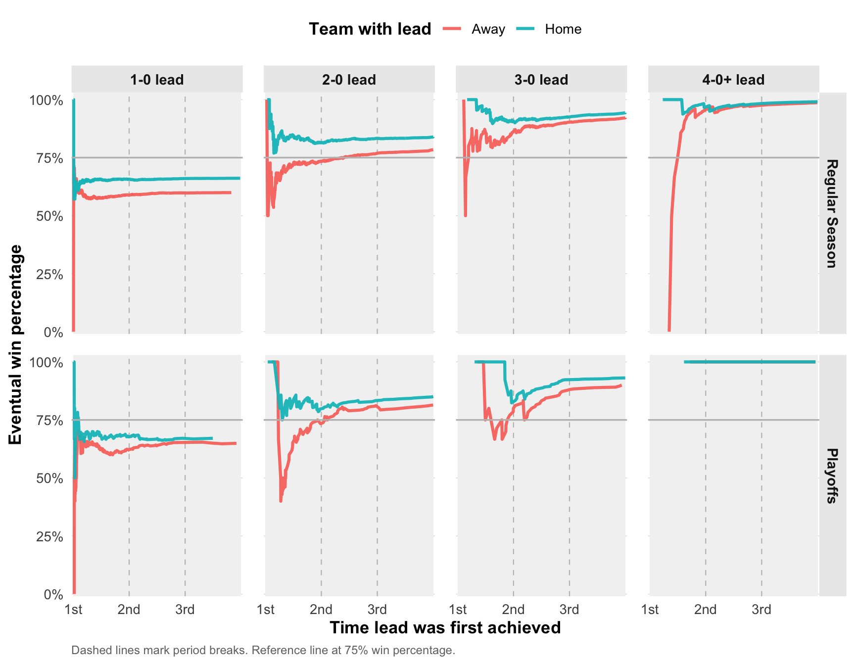
Note: One thing to keep in mind in interpreting these plots is that the sample size accumulates with the progression of the game. The rates are unstable at the start (and stabilize throughout) because we’re computing the win rate of those games where a lead was achieved by that time in the game. By definition, the first rate will be based on a sample size of N=1, then N=2, etc.

First, we can see that in general, for any particular lead, the win percentage is higher the later in the game the lead is achieved. This obviously makes sense because the other team has less time to come back. Another (maybe expected) result is that the home team general wins more often when a lead is obtained compared to the away team, and this difference is roughly similar for regular season and playoff games.

More direct to our questions of interest: we can see that for away teams specifically, even a mid-to-late first period two-goal lead isn’t really securing any win. Especially in playoffs, even a 3 goal lead doesn’t make much of a difference there (compared to two goals). We don’t see this for the home team, which might indicate a real home ice advantage when a lead is taken. It’s also clear that getting the 2 or 3 goal lead in the mid-to-late second period is really where the win percentage starts to plateau. What’s particularly interesting is that, for away teams in playoffs, a 3 goal lead towards the end of first period does not seem to be much different from a 2 goal lead in terms of win rate (albeit the sample sizes are sort of small here).

2. Comeback rate by timing of lead

Next, we’ll do something similar to the previous metric, but instead of win percentage, we’ll look at the comeback rate. Once a certain lead is obtained, a comeback will be indicated as the earliest future point in the game where the score is tied again. We’ll again repeat this analysis for both lead definitions.

Shutout leads

comeback_pct_shutout <-
  goals |>

    # Sort the data
    arrange(
      GameID,
      Period,
      Time
    ) |>

    # Count the cumulative goals for each team throughout the game
    mutate(
      HomeGoals = cumsum(ScoringTeam == "Home"),
      AwayGoals = cumsum(ScoringTeam == "Away"),
      .by = GameID
    ) |>

    # Determine which team had the desired lead (and when)
    mutate(
      LeadTeam = case_when(
        HomeGoals == 0 & AwayGoals > 0 ~ "Away",
        HomeGoals > 0 & AwayGoals == 0 ~ "Home",
        TRUE ~ NA_character_
      )
    ) |>

    # Filter out other scores
    filter(!is.na(LeadTeam)) |>

    # Compute the lead
    mutate(
      Lead = pmax(HomeGoals, AwayGoals)
    ) |>

    # Keep a few columns
    select(
      GameID,
      Time,
      LeadTeam,
      Lead
    ) |>
    
    # Join to indicate when it was tied
    left_join(
      y = 
        goals |>

        # Sort the data
        arrange(
          GameID,
          Period,
          Time
        ) |>

        # Count the cumulative goals for each team throughout the game
        mutate(
          HomeGoals = cumsum(ScoringTeam == "Home"),
          AwayGoals = cumsum(ScoringTeam == "Away"),
          .by = GameID
        ) |>
        
        # Filter to when the games are tied
        filter(HomeGoals == AwayGoals) |>
          
        # Keep a few columns
        select(
          GameID,
          Lead = HomeGoals,
          ComebackTime = Time
        ),
      by = 
        c(
          "GameID",
          "Lead"
        )
    ) |>
    
    # Indicate if a comeback occurred
    mutate(
      Lead = case_when(
        Lead >= 4 ~ "4-0+",
        TRUE ~ paste0(Lead, "-0")
      ),
      Comeback = as.numeric(!is.na(ComebackTime))
    ) |>
    
    # Join to get game outcomes
    inner_join(
      y = games,
      by = "GameID"
    ) |>

    # Sort the data
    arrange(PlayoffGame, LeadTeam, Lead, Time) |>

    # Count the cumulative comebacks
    mutate(
      TotalComebacks = cumsum(Comeback),
      TotalGames = 1,
      TotalGames = cumsum(TotalGames),
      .by = c(
        PlayoffGame,
        LeadTeam,
        Lead
      )
    ) |>

    # Add some clean plot labels
    mutate(
      ComebackPct = TotalComebacks / TotalGames,
      Minute = Time / 60,
      Lead = factor(Lead),
      LeadTeam = factor(LeadTeam),
      PlayoffGame = factor(PlayoffGame),
      PlayoffGame = fct_recode(
        PlayoffGame,
        `Regular Season` = "0",
        Playoffs = "1"
      )
    ) |>

    # Filter to regulation goals only
    filter(Time <= 3600)

In this analysis, there are 13207 lead timepoints across 6963 games. The following table shows this broken down game type, which team had the lead, and lead amount.

Use arrows to expand the table

comeback_pct_shutout |>

  # Indicate period
  mutate(
    Period = 
      case_when(
        Time <= 1200 ~ 1,
        Time <= 2400 ~ 2,
        Time <= 3600 ~ 3
      )
  ) |>

  # Make metrics
  summarize(
    Leads = n(),
    Games = n_distinct(GameID),
    ComebackRate = mean(Comeback),
    .by = 
      c(
        PlayoffGame,
        LeadTeam,
        Period,
        Lead
      )
  ) |>
  
  # Make table
  reactable(
    groupBy = c("PlayoffGame", "LeadTeam", "Period"),
    columns = 
      list(
        PlayoffGame = colDef(name = "Game Type", align = "left"),
        LeadTeam = colDef(name = "Lead Team", align = "left"),
        Leads = colDef(name = "Lead Timepoints", align = "center", aggregate = "sum"),
        ComebackRate = colDef(name = "Comeback Rate %", align = "center", aggregate = zildge::rectbl_agg_wtd("Leads"), format = colFormat(digits = 2, percent = TRUE))
      ),
    resizable = TRUE,
    sortable = TRUE,
    theme = reactablefmtr::minty()
  )

Now we can evaluate the comeback rate by game time.

comeback_pct_shutout |>

  # Make a plot
  ggplot(aes(x = Minute, y = ComebackPct, color = LeadTeam)) +
  geom_rect(
    data = period_bands,
    aes(xmin = xmin, xmax = xmax, ymin = ymin, ymax = ymax),
    inherit.aes = FALSE,
    fill = "grey95",
    color = NA
  ) +
  geom_vline(
    xintercept = c(20, 40),
    color = "grey75",
    linewidth = 0.4,
    linetype = "dashed"
  ) +
  geom_line(linewidth = 1.1, alpha = 0.95) +
  geom_hline(yintercept = .25, color = "gray") +
  facet_grid(
    PlayoffGame ~ Lead,
    labeller = labeller(
      Lead = function(x) paste0(x, " lead")
    )
  ) +
  scale_y_continuous(
    labels = percent_format(accuracy = 1),
    limits = c(0, 1),
    breaks = seq(0, 1, 0.25),
    expand = expansion(mult = c(0.01, 0.03))
  ) +
  scale_x_continuous(
    breaks = c(0, 20, 40, 60),
    labels = c("1st", "2nd", "3rd", ""),
    limits = c(0, 60),
    expand = expansion(mult = c(0.01, 0.01))
  ) +
  labs(
    x = "Time lead was first achieved",
    y = "Eventual comeback rate of opposing team",
    color = "Team with lead",
    caption = "Dashed lines mark period breaks. Reference line at 25% comeback rate."
  ) +
  theme_minimal(base_size = 13) +
  theme(
    plot.title = element_text(face = "bold", size = 20),
    plot.subtitle = element_text(
      size = 12,
      color = "grey35",
      margin = margin(b = 12)
    ),
    plot.caption = element_text(color = "grey45", size = 9, hjust = 0),
    legend.position = "top",
    legend.title = element_text(face = "bold"),
    panel.grid.minor = element_blank(),
    panel.grid.major.x = element_blank(),
    panel.grid.major.y = element_line(color = "grey88", linewidth = 0.3),
    strip.text = element_text(face = "bold", size = 11),
    strip.background = element_rect(fill = "grey92", color = NA),
    panel.spacing = unit(1.1, "lines"),
    axis.title = element_text(face = "bold"),
    axis.text = element_text(color = "grey30")
  )

Differential leads

comeback_pct_differential <-
  goals |>

    # Sort the data
    arrange(
      GameID,
      Period,
      Time
    ) |>

    # Count the cumulative goals for each team throughout the game
    mutate(
      HomeGoals = cumsum(ScoringTeam == "Home"),
      AwayGoals = cumsum(ScoringTeam == "Away"),
      .by = GameID
    ) |>

    # Determine which team had the desired lead (and when)
    mutate(
      LeadTeam = case_when(
        AwayGoals > HomeGoals ~ "Away",
        HomeGoals > AwayGoals ~ "Home",
        TRUE ~ NA_character_
      )
    ) |>

    # Filter out other scores
    filter(!is.na(LeadTeam)) |>

    # Compute the lead
    mutate(
      Lead = abs(HomeGoals - AwayGoals),
      LeadTeamGoals = pmax(HomeGoals, AwayGoals)
    ) |>

    # Keep a few columns
    select(
      GameID,
      Time,
      LeadTeam,
      Lead,
      LeadTeamGoals
    ) |>
    
    # Make join key
    mutate(JoinTeam = case_when(LeadTeam == "Away" ~ "Home", TRUE ~ "Away")) |>
    
    # Join to indicate when comeback occurred
    left_join(
      y = 
        goals |>

        # Sort the data
        arrange(
          GameID,
          Period,
          Time
        ) |>

        # Count the cumulative goals for each team throughout the game
        mutate(
          HomeGoals = cumsum(ScoringTeam == "Home"),
          AwayGoals = cumsum(ScoringTeam == "Away"),
          .by = GameID
        ) |>
        
        # Rename the columns
        rename(Home = HomeGoals, Away = AwayGoals) |>

        # Filter to points in the game where it was tied
        filter(Home == Away) |>
        
        # Send down the rows
        pivot_longer(
          cols = c(Home, Away),
          names_to = "JoinTeam",
          values_to = "Goals"
        ) |>
        
        # Find the earliest time each team had that many goals
        summarize(
          ComebackTime = min(Time),
          .by = 
            c(
              GameID,
              JoinTeam,
              Goals
            )
        ),
      by = 
        c(
          "GameID",
          "JoinTeam",
          "LeadTeamGoals" = "Goals"
        )
    ) |>
    
    # Indicate if a comeback occurred
    mutate(
      Lead = case_when(
        Lead >= 4 ~ "4+",
        TRUE ~ as.character(Lead)
      ),
      Comeback = as.numeric(!is.na(ComebackTime))
    ) |>
    
    # Join to get game outcomes
    inner_join(
      y = games,
      by = "GameID"
    ) |>

    # Sort the data
    arrange(PlayoffGame, LeadTeam, Lead, Time) |>

    # Count the cumulative comebacks
    mutate(
      TotalComebacks = cumsum(Comeback),
      TotalGames = 1,
      TotalGames = cumsum(TotalGames),
      .by = c(
        PlayoffGame,
        LeadTeam,
        Lead
      )
    ) |>

    # Add some clean plot labels
    mutate(
      ComebackPct = TotalComebacks / TotalGames,
      Minute = Time / 60,
      Lead = factor(Lead),
      LeadTeam = factor(LeadTeam),
      PlayoffGame = factor(PlayoffGame),
      PlayoffGame = fct_recode(
        PlayoffGame,
        `Regular Season` = "0",
        Playoffs = "1"
      )
    ) |>

    # Filter to regulation goals only
    filter(Time <= 3600)

In this analysis, there are 34391 lead timepoints across 6963 games. The following table shows this broken down game type, which team had the lead, and lead amount.

Use arrows to expand the table

comeback_pct_differential |>

  # Indicate period
  mutate(
    Period = 
      case_when(
        Time <= 1200 ~ 1,
        Time <= 2400 ~ 2,
        Time <= 3600 ~ 3
      )
  ) |>

  # Make metrics
  summarize(
    Leads = n(),
    Games = n_distinct(GameID),
    ComebackRate = mean(Comeback),
    .by = 
      c(
        PlayoffGame,
        LeadTeam,
        Period,
        Lead
      )
  ) |>
  
  # Make table
  reactable(
    groupBy = c("PlayoffGame", "LeadTeam", "Period"),
    columns = 
      list(
        PlayoffGame = colDef(name = "Game Type", align = "left"),
        LeadTeam = colDef(name = "Lead Team", align = "left"),
        Leads = colDef(name = "Lead Timepoints", align = "center", aggregate = "sum"),
        ComebackRate = colDef(name = "Comeback Rate %", align = "center", aggregate = zildge::rectbl_agg_wtd("Leads"), format = colFormat(digits = 2, percent = TRUE))
      ),
    resizable = TRUE,
    sortable = TRUE,
    theme = reactablefmtr::minty()
  )

Now we can evaluate the comeback rate by game time.

comeback_pct_differential |>

  # Make a plot
  ggplot(aes(x = Minute, y = ComebackPct, color = LeadTeam)) +
  geom_rect(
    data = period_bands,
    aes(xmin = xmin, xmax = xmax, ymin = ymin, ymax = ymax),
    inherit.aes = FALSE,
    fill = "grey95",
    color = NA
  ) +
  geom_vline(
    xintercept = c(20, 40),
    color = "grey75",
    linewidth = 0.4,
    linetype = "dashed"
  ) +
  geom_line(linewidth = 1.1, alpha = 0.95) +
  geom_hline(yintercept = .25, color = "gray") +
  facet_grid(
    PlayoffGame ~ Lead,
    labeller = labeller(
      Lead = function(x) paste0(x, " goal lead")
    )
  ) +
  scale_y_continuous(
    labels = percent_format(accuracy = 1),
    limits = c(0, 1),
    breaks = seq(0, 1, 0.25),
    expand = expansion(mult = c(0.01, 0.03))
  ) +
  scale_x_continuous(
    breaks = c(0, 20, 40, 60),
    labels = c("1st", "2nd", "3rd", ""),
    limits = c(0, 60),
    expand = expansion(mult = c(0.01, 0.01))
  ) +
  labs(
    x = "Time lead was first achieved",
    y = "Eventual comeback rate of opposing team",
    color = "Team with lead",
    caption = "Dashed lines mark period breaks. Reference line at 25% comeback rate."
  ) +
  theme_minimal(base_size = 13) +
  theme(
    plot.title = element_text(face = "bold", size = 20),
    plot.subtitle = element_text(
      size = 12,
      color = "grey35",
      margin = margin(b = 12)
    ),
    plot.caption = element_text(color = "grey45", size = 9, hjust = 0),
    legend.position = "top",
    legend.title = element_text(face = "bold"),
    panel.grid.minor = element_blank(),
    panel.grid.major.x = element_blank(),
    panel.grid.major.y = element_line(color = "grey88", linewidth = 0.3),
    strip.text = element_text(face = "bold", size = 11),
    strip.background = element_rect(fill = "grey92", color = NA),
    panel.spacing = unit(1.1, "lines"),
    axis.title = element_text(face = "bold"),
    axis.text = element_text(color = "grey30")
  )

Noteworthy observations

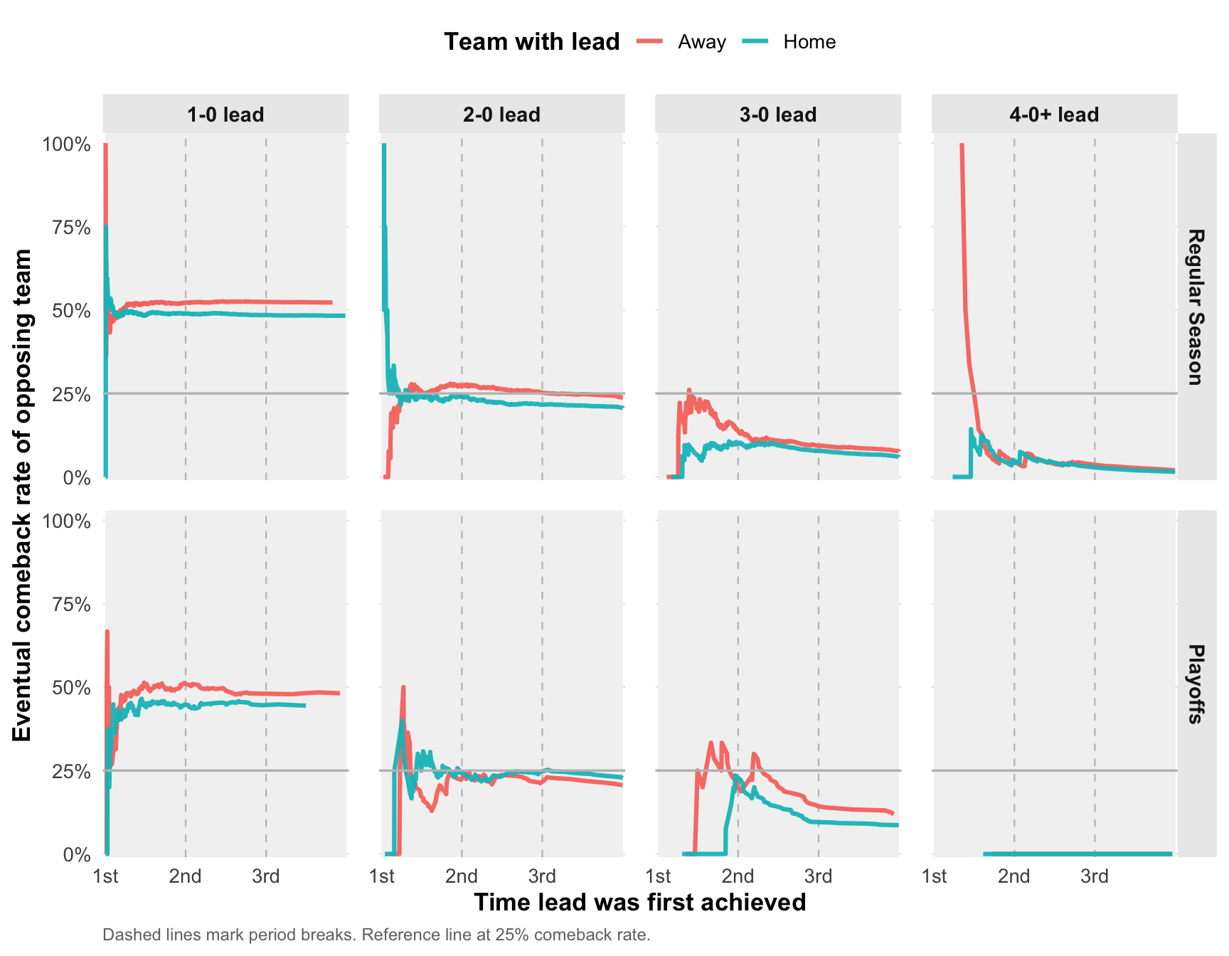
In some ways this is a reverse image of the win percentage metric, but there are some additional interesting findings here. Specifically for playoff games, looking at the table above, we can see that comeback rates are basically the same for a 2-0 or a 3-0 lead taken in the first period, regardless if it’s the home or away team (in fact, the home allows for a slightly higher rate of comebacks). But when you move on to periods 2 and 3, the differences in comeback rates between a 2 and 3 goal lead are huge. This is also supported by the plots showing lead timing. This seems to suggest that, on average, there isn’t a substantial difference in having a 2 goal lead versus 3 goal lead in the first period (in the playoffs). However, in the regular season, there is a huge difference.

3. Win percentage by lead and comeback time

Finally, putting these two concepts together, an interesting question is how the win rates differ by how big the lead was and when the comeback occurred. You might argue that an earlier comeback sort of “resets” the game with a lot of gameplay to be had, whereas a later comeback might signal more momentum for the opposing team, which may end up closing it out with a win. Let’s see what the data shows. Here we’ll just focus on the shutout leads.

win_comeback_shutout <-
  win_pct_shutout |>

    # Keep a few columns
    select(
      GameID,
      Time,
      LeadTeam,
      Lead,
      PlayoffGame,
      LeadTeamWon
    ) |>
    
    # Join to get comeback time
    inner_join(
      y = 
        comeback_pct_shutout |>
        select(
          GameID,
          Time,
          Lead,
          ComebackTime
        ),
      by = 
        c(
          "GameID",
          "Time",
          "Lead"
        )
    ) |>
    
    # Filter where a comeback occurred
    filter(!is.na(ComebackTime)) |>
  
    # Sort the data
    arrange(PlayoffGame, LeadTeam, Lead, Time) |>

    # Count the cumulative wins over the game
    mutate(
      TotalWins = cumsum(LeadTeamWon),
      TotalGames = 1,
      TotalGames = cumsum(TotalGames),
      .by = c(
        PlayoffGame,
        LeadTeam,
        Lead
      )
    ) |>

    # Add some clean plot labels
    mutate(
      WinPct = TotalWins / TotalGames,
      Minute = Time / 60
    ) |>
  
    # Filter to regulation goals only
    filter(Time <= 3600)

Win rates after coming back

First, let’s just look at what the overall win percentages are for teams that allow a comeback to occur (again, by the amount of the lead and whether it’s a regular season or playoff game). In this analysis, there are 4367 lead timepoints, where team who had the lead won 1915 (43.9%) of the time, across 4367 games.

Use arrows to expand the table

win_comeback_shutout |>

  # Indicate period
  mutate(
    Period = 
      case_when(
        Time <= 1200 ~ 1,
        Time <= 2400 ~ 2,
        Time <= 3600 ~ 3
      )
  ) |>

  # Make metrics
  summarize(
    Leads = n(),
    Games = n_distinct(GameID),
    WinRate = mean(LeadTeamWon),
    .by = 
      c(
        PlayoffGame,
        LeadTeam,
        Period,
        Lead
      )
  ) |>
  
  # Make table
  reactable(
    groupBy = c("PlayoffGame", "LeadTeam", "Period"),
    columns = 
      list(
        PlayoffGame = colDef(name = "Game Type", align = "left"),
        LeadTeam = colDef(name = "Lead Team", align = "left"),
        Leads = colDef(name = "Lead Timepoints", align = "center", aggregate = "sum"),
        WinRate = colDef(name = "Win %", align = "center", aggregate = zildge::rectbl_agg_wtd("Leads"), format = colFormat(digits = 2, percent = TRUE))
      ),
    resizable = TRUE,
    sortable = TRUE,
    theme = reactablefmtr::minty()
  )

Now we can analogously look at the plot.

win_comeback_shutout |>

  # Make a plot
  ggplot(aes(x = Minute, y = WinPct, color = LeadTeam)) +
  geom_rect(
    data = period_bands,
    aes(xmin = xmin, xmax = xmax, ymin = ymin, ymax = ymax),
    inherit.aes = FALSE,
    fill = "grey95",
    color = NA
  ) +
  geom_vline(
    xintercept = c(20, 40),
    color = "grey75",
    linewidth = 0.4,
    linetype = "dashed"
  ) +
  geom_line(linewidth = 1.1, alpha = 0.95) +
  geom_hline(yintercept = .50, color = "gray") +
  facet_grid(
    PlayoffGame ~ Lead,
    labeller = labeller(
      Lead = function(x) paste0(x, " lead")
    )
  ) +
  scale_y_continuous(
    labels = percent_format(accuracy = 1),
    limits = c(0, 1),
    breaks = seq(0, 1, 0.25),
    expand = expansion(mult = c(0.01, 0.03))
  ) +
  scale_x_continuous(
    breaks = c(0, 20, 40, 60),
    labels = c("1st", "2nd", "3rd", ""),
    limits = c(0, 60),
    expand = expansion(mult = c(0.01, 0.01))
  ) +
  labs(
    x = "Time lead was first achieved",
    y = "Eventual win percentage after opposition comeback",
    color = "Team with lead",
    caption = "Dashed lines mark period breaks. Reference line at 50% win percentage."
  ) +
  theme_minimal(base_size = 13) +
  theme(
    plot.title = element_text(face = "bold", size = 20),
    plot.subtitle = element_text(
      size = 12,
      color = "grey35",
      margin = margin(b = 12)
    ),
    plot.caption = element_text(color = "grey45", size = 9, hjust = 0),
    legend.position = "top",
    legend.title = element_text(face = "bold"),
    panel.grid.minor = element_blank(),
    panel.grid.major.x = element_blank(),
    panel.grid.major.y = element_line(color = "grey88", linewidth = 0.3),
    strip.text = element_text(face = "bold", size = 11),
    strip.background = element_rect(fill = "grey92", color = NA),
    panel.spacing = unit(1.1, "lines"),
    axis.title = element_text(face = "bold"),
    axis.text = element_text(color = "grey30")
  )

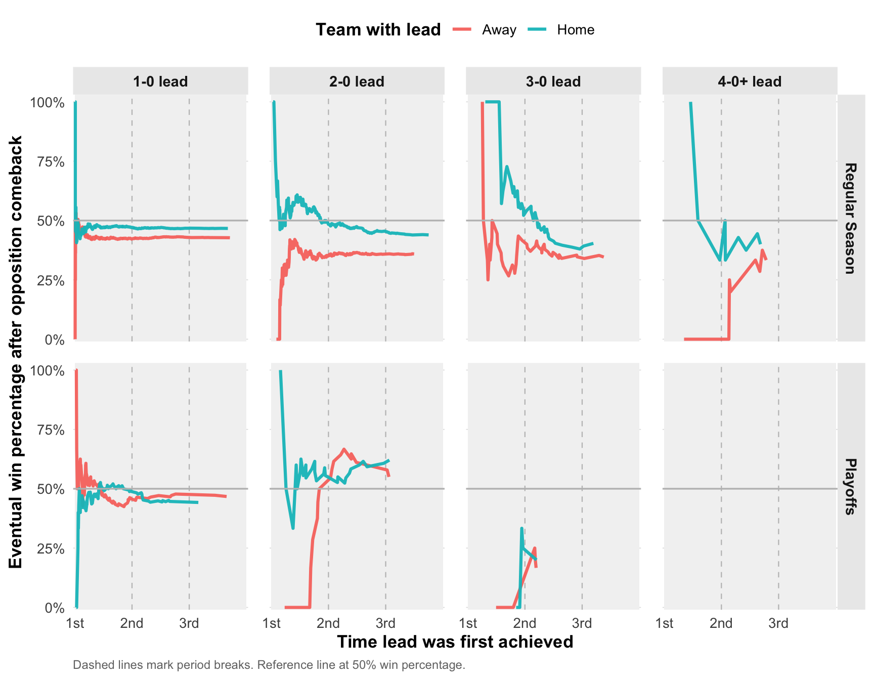
Overall when a comeback occurs, the team with the original team wins a little less than half the time. What’s somewhat interesting is that these rates are somewhat stable over the game. For example, when the team with a 2-0 allows a comeback, it didn’t really matter when their original 2-0 lead occured (at least in regular season). There’s still a difference between home and away teams, and a bit of a flipped dynamic for late first period 1-0 leads.

Win rates accounting for comeback time

Lastly, we’ll try to understand a little bit if the time at which the comeback occurred says anything about the win rate.

# Periods
period_levels <- c("1st", "2nd", "3rd")

# Plot data
heatmap_df <- 
  win_comeback_shutout |>

  # Filter to regulation
  filter(Time <= 3600, ComebackTime <= 3600) |>
  
  # Make bins
  mutate(
    LeadPeriod = case_when(
      Time <= 1200 ~ "1st",
      Time <= 2400 ~ "2nd",
      Time <= 3600 ~ "3rd"
    ) |> factor(levels = period_levels),

    ComebackPeriod = case_when(
      ComebackTime <= 1200 ~ "1st",
      ComebackTime <= 2400 ~ "2nd",
      ComebackTime <= 3600 ~ "3rd"
    ) |> factor(levels = period_levels)
  ) |>
  
  # Compute metrics
  summarize(
    Games = n(),
    WinRate = mean(LeadTeamWon),
    .by = c(
      PlayoffGame,
      LeadTeam,
      Lead,
      LeadPeriod,
      ComebackPeriod
    )
  )

# Make plot
ggplot(
  heatmap_df,
  aes(
    x = LeadPeriod,
    y = ComebackPeriod,
    fill = WinRate
  )
) +
  geom_tile(color = "white", linewidth = 1) +
  geom_text(
    aes(label = paste0(percent(WinRate, accuracy = 1), "\n(n=", Games, ")")),
    size = 3.2,
    fontface = "bold",
    color = "grey15"
  ) +
  facet_grid(
    PlayoffGame + LeadTeam ~ Lead
  ) +
  scale_fill_gradient2(
    low = "#b2182b",
    mid = "white",
    high = "#2166ac",
    midpoint = 0.5,
    limits = c(0, 1),
    labels = percent_format(accuracy = 1)
  ) +
  labs(
    x = "Period when original lead was obtained",
    y = "Period when comeback occurred",
    fill = "Original lead\nteam win rate"
  ) +
  theme_minimal(base_size = 13) +
  theme(
    plot.title = element_text(face = "bold", size = 18),
    plot.subtitle = element_text(color = "grey35"),
    panel.grid = element_blank(),
    axis.title = element_text(face = "bold"),
    strip.text = element_text(face = "bold"),
    strip.background = element_rect(fill = "grey92", color = NA),
    legend.position = "right"
  )

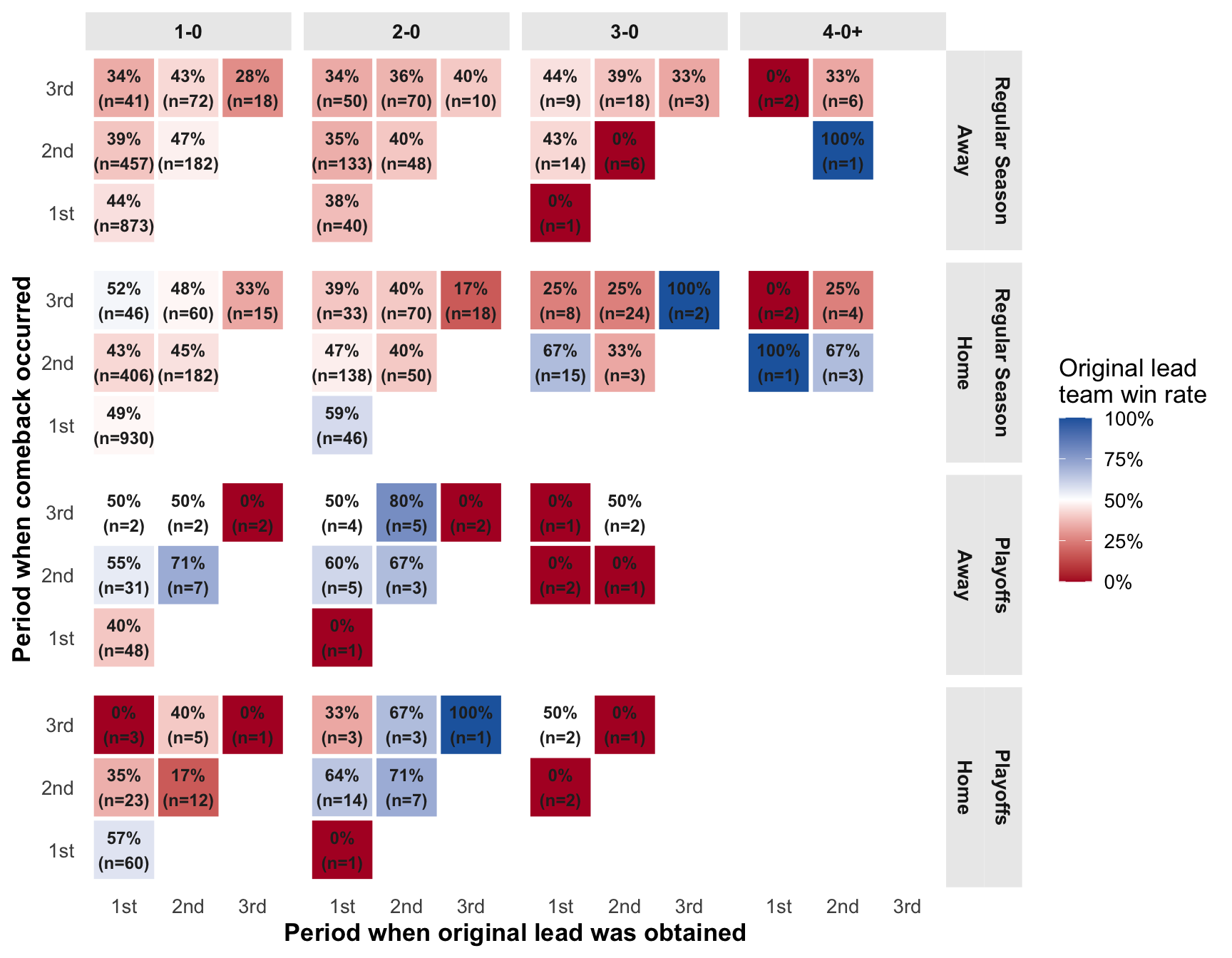
There is a lot going on here, so we’ll not read too much into it.

Conclusion (so far)

We are obviously just scratching the surface of where we could take this analysis, but we’ve at least gotten a look at some high-level relevant insights to create a foundational understanding. My biggest takeaway so far, as it relates to the primary question, is that on average there is questionable added utility of a 3-0 lead (or any 3-goal lead) in the first period, compared to a 2-goal lead, specifically in the playoffs (and maybe even more specifically for road teams). However, overall attaining a larger lead throughout the game clearly pays off, so teams should still keep scoring goals.